Added addendum
Source Link
Michael E2
  • 244.7k
  • 18
  • 351
  • 774

The SVD of a real symmetric matrix $A$ is simple, fast, accurate way to get $X$ and $B$ (and $A$ need not be invertible):

cj = u2\[Transpose] . conj . u1;
conj - u2 . cj . u1\[Transpose] // Norm
(*  9.36499*10^-16  *)

Addendum 2

Perhaps the efficiency of SingularValueDecomposition on numerical problems is not widely appreciated. It is much more accurate than the Inverse/MatrixPower power approach and quite a bit faster. Here is a code for comparing the two methods. (Takes about a minute to run for 100 data points.)

SeedRandom[3];
(data = Transpose[#, {3, 1, 2}] &@Table[
      (* Set up: random symm. mat. of random sizes *)
      n = RandomInteger[{2, 800}];
      amat = #\[Transpose] . # &@RandomReal[{-1, 1}, {n, n}];
      conj = Orthogonalize@RandomReal[{-1, 1}, {n, n}];
      bmat = conj . amat . conj\[Transpose];
      (* SVD *)
      t1 = (v1 = Last@SingularValueDecomposition[amat];
          v2 = Last@SingularValueDecomposition[bmat];
          xmat1 = v2 . v1\[Transpose];) // AbsoluteTiming // First;
      (* Inverse *)
      t2 = (xmat2 = 
            bmat . MatrixPower[Inverse[bmat] . Inverse[amat], 1/2];) //
          AbsoluteTiming // First;
      {{{n, 
         Norm[xmat1 . amat . xmat1\[Transpose] - bmat]/
          Norm[amat]}, {n, 
         Norm[xmat2 . amat . xmat2\[Transpose] - bmat]/Norm[amat]}},
       {{n, t1}, {n, t2}}},
      {100}]) //
  MapThread[ListLogPlot[#,
      Frame -> True,
      FrameLabel -> {"Dimension", #2},
      PlotLegends -> {"SVD", "Inverse"}] &,
    {#, {"Relative Error (2-norm)", "Timing"}}] &

Inverse throws a few warnings:

...
Inverse::luc: Result for Inverse of badly conditioned matrix {<<1>>} may contain significant numerical errors.
...
General::stop: Further output of Inverse::luc will be suppressed during this calculation.

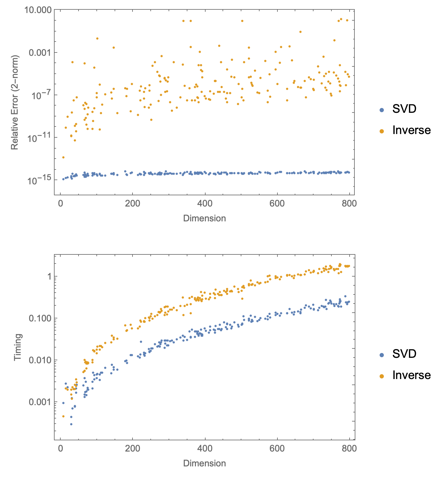
The first plot shows the relative error of the two methods on random matrices versus dimension. It illustrates the stability of the SVD method. The second shows the time each run took.

Mathematica graphics

The SVD of a real symmetric matrix $A$ is simple way to get $X$ and $B$ (and $A$ need not be invertible):

cj = u2\[Transpose] . conj . u1;
conj - u2 . cj . u1\[Transpose] // Norm
(*  9.36499*10^-16  *)

The SVD of a real symmetric matrix $A$ is simple, fast, accurate way to get $X$ and $B$ (and $A$ need not be invertible):

cj = u2\[Transpose] . conj . u1;
conj - u2 . cj . u1\[Transpose] // Norm
(*  9.36499*10^-16  *)

Addendum 2

Perhaps the efficiency of SingularValueDecomposition on numerical problems is not widely appreciated. It is much more accurate than the Inverse/MatrixPower power approach and quite a bit faster. Here is a code for comparing the two methods. (Takes about a minute to run for 100 data points.)

SeedRandom[3];
(data = Transpose[#, {3, 1, 2}] &@Table[
      (* Set up: random symm. mat. of random sizes *)
      n = RandomInteger[{2, 800}];
      amat = #\[Transpose] . # &@RandomReal[{-1, 1}, {n, n}];
      conj = Orthogonalize@RandomReal[{-1, 1}, {n, n}];
      bmat = conj . amat . conj\[Transpose];
      (* SVD *)
      t1 = (v1 = Last@SingularValueDecomposition[amat];
          v2 = Last@SingularValueDecomposition[bmat];
          xmat1 = v2 . v1\[Transpose];) // AbsoluteTiming // First;
      (* Inverse *)
      t2 = (xmat2 = 
            bmat . MatrixPower[Inverse[bmat] . Inverse[amat], 1/2];) //
          AbsoluteTiming // First;
      {{{n, 
         Norm[xmat1 . amat . xmat1\[Transpose] - bmat]/
          Norm[amat]}, {n, 
         Norm[xmat2 . amat . xmat2\[Transpose] - bmat]/Norm[amat]}},
       {{n, t1}, {n, t2}}},
      {100}]) //
  MapThread[ListLogPlot[#,
      Frame -> True,
      FrameLabel -> {"Dimension", #2},
      PlotLegends -> {"SVD", "Inverse"}] &,
    {#, {"Relative Error (2-norm)", "Timing"}}] &

Inverse throws a few warnings:

...
Inverse::luc: Result for Inverse of badly conditioned matrix {<<1>>} may contain significant numerical errors.
...
General::stop: Further output of Inverse::luc will be suppressed during this calculation.

The first plot shows the relative error of the two methods on random matrices versus dimension. It illustrates the stability of the SVD method. The second shows the time each run took.
Mathematica graphics

Added addendum
Source Link
Michael E2
  • 244.7k
  • 18
  • 351
  • 774

The SVD of a real symmetric matrix $A$ yieldsis simple way to get $X$ and $B$ (and $A$ need not be invertible):

(* set up *)
SeedRandom[0];
amat = #\[Transpose] . # &@RandomReal[{-1, 1}, {5, 5}]; 

(* solution *)
{xmat, bmat} = Most@SingularValueDecomposition[amat];
xmat = xmat\[Transpose];

Check:

Chop[xmat . amat . xmat\[Transpose]] == bmat
(*  True  *)

xmat . amat . xmat\[Transpose] // Threshold // MatrixForm
bmat // MatrixForm

Addendum

It should be clear that the above may be adapted to the original problem statement, amended with the suitable hypotheses:

Given two real, symmetric, orthogonally-similar matrices $A$ and $B$, not necessarily invertible, find an orthogonal matrix $X$ such that $X.A.X^t=B$.

(* set up: 5x5, rank 4 *)
SeedRandom[2];
amat = #\[Transpose] . # &@RandomReal[{-1, 1}, {4, 5}];
conj = Orthogonalize@RandomReal[{-1, 1}, {5, 5}];
bmat = conj . amat . conj\[Transpose];

(* solution *)
u1 = First@SingularValueDecomposition[amat];
u2 = First@SingularValueDecomposition[bmat];
xmat = u2 . u1\[Transpose];

Check:

Norm[xmat . amat . xmat\[Transpose] - bmat]/Norm[amat]
(*  3.12068*10^-16  *)

Since u1 and u2 are not unique, xmat is not necessarily the same as conj, and the solution xmat is unique only up to the uniqueness of the SVD. Given another solution such as conj, one can find its relationship to u1 and u2 as follows:

cj = u2\[Transpose] . conj . u1;
conj - u2 . cj . u1\[Transpose] // Norm
(*  9.36499*10^-16  *)

The SVD of a real symmetric matrix $A$ yields $X$ and $B$:

SeedRandom[0];
amat = #\[Transpose] . # &@RandomReal[{-1, 1}, {5, 5}];
{xmat, bmat} = Most@SingularValueDecomposition[amat];
xmat = xmat\[Transpose];

Check:

Chop[xmat . amat . xmat\[Transpose]] == bmat
(*  True  *)

xmat . amat . xmat\[Transpose] // Threshold // MatrixForm
bmat // MatrixForm

The SVD of a real symmetric matrix $A$ is simple way to get $X$ and $B$ (and $A$ need not be invertible):

(* set up *)
SeedRandom[0];
amat = #\[Transpose] . # &@RandomReal[{-1, 1}, {5, 5}]; 

(* solution *)
{xmat, bmat} = Most@SingularValueDecomposition[amat];
xmat = xmat\[Transpose];

Check:

Chop[xmat . amat . xmat\[Transpose]] == bmat
(*  True  *)

xmat . amat . xmat\[Transpose] // Threshold // MatrixForm
bmat // MatrixForm

Addendum

It should be clear that the above may be adapted to the original problem statement, amended with the suitable hypotheses:

Given two real, symmetric, orthogonally-similar matrices $A$ and $B$, not necessarily invertible, find an orthogonal matrix $X$ such that $X.A.X^t=B$.

(* set up: 5x5, rank 4 *)
SeedRandom[2];
amat = #\[Transpose] . # &@RandomReal[{-1, 1}, {4, 5}];
conj = Orthogonalize@RandomReal[{-1, 1}, {5, 5}];
bmat = conj . amat . conj\[Transpose];

(* solution *)
u1 = First@SingularValueDecomposition[amat];
u2 = First@SingularValueDecomposition[bmat];
xmat = u2 . u1\[Transpose];

Check:

Norm[xmat . amat . xmat\[Transpose] - bmat]/Norm[amat]
(*  3.12068*10^-16  *)

Since u1 and u2 are not unique, xmat is not necessarily the same as conj, and the solution xmat is unique only up to the uniqueness of the SVD. Given another solution such as conj, one can find its relationship to u1 and u2 as follows:

cj = u2\[Transpose] . conj . u1;
conj - u2 . cj . u1\[Transpose] // Norm
(*  9.36499*10^-16  *)
Source Link
Michael E2
  • 244.7k
  • 18
  • 351
  • 774

The SVD of a real symmetric matrix $A$ yields $X$ and $B$:

SeedRandom[0];
amat = #\[Transpose] . # &@RandomReal[{-1, 1}, {5, 5}];
{xmat, bmat} = Most@SingularValueDecomposition[amat];
xmat = xmat\[Transpose];

Check:

Chop[xmat . amat . xmat\[Transpose]] == bmat
(*  True  *)

xmat . amat . xmat\[Transpose] // Threshold // MatrixForm
bmat // MatrixForm