0
$\begingroup$

I am trying to fit the following data (called TflogqIND):

TflogqIND={{0., 36.4886}, {Log[2]/Log[10], 37.1485}, {Log[5]/Log[10], 
  38.3859}, {1, 39.2263}, {Log[20]/Log[10], 39.8772}, {Log[30]/
  Log[10], 40.0107}}

to the following equation:

 eqn = ((log10q - Log10[qref]) == 
       c1*(Tfp - Tfpref)/(c2 + (Tfp - Tfpref))); (*WLF equation*)
    model = Tfp /. Solve[eqn, Tfp][[1]] // FullSimplify;
    constIND = {Tfpref -> 39.2263, 
       qref -> 10};
    modelIND = model /. (constIND // Rationalize) // FullSimplify;
    
    nlmIND = NonlinearModelFit[
       TflogqIND, {modelIND, c1 > 5, c2 > 5}, {c1, c2}, log10q]; 

As you can see from plotting:

Show[ ListPlot[TflogqIND, PlotMarkers -> Style[\[FilledSquare], 18, Red], Frame -> True, Axes -> False, FrameStyle -> 16, LabelStyle -> {Black, Bold, 10}, ImageSize -> Large, GridLines -> Automatic, GridLinesStyle -> Lighter[Gray, .8], PlotRange -> All], Plot[nlmIND[log10q], {log10q, 0, 1.4}, PlotStyle -> {Red, Dashed}]]

The model seems to describe the data well. However, the parameters (obtained from nlmIND["BestFitParameters"] with {c1 -> 1331.87, c2 -> 3520.53}) don't make any sense. Usually c1 and c2 parameters are from 1 to around 100 or 200 at the most.

I think there must be a mistake somewhere but I cannot see it. How can I fix the model to give better c1 and c2 values and better describe the data using that equation?

$\endgroup$
2
  • 1
    $\begingroup$ "Usually c1 and c2 parameters are from 1 to around 100 or 200 at the most." - then you should have put a constraint like that in your fit, no? {modelIND, 200 > c1 > 5, 200 > c2 > 5} Also, you would still want a way to figure out good initial values for these parameters. $\endgroup$ Commented Jan 11, 2021 at 7:31
  • 3
    $\begingroup$ For this particular dataset and model there is no finite set of parameter estimates that maximizes the likelihood or minimizes the mean square error. The estimate for c1 can be found in terms of c2 but then the mean square error keeps getting smaller for increasing values of c2. I'll write up the details tomorrow as it's too late at night for me to do so now. $\endgroup$
    – JimB
    Commented Jan 11, 2021 at 7:50

1 Answer 1

3
$\begingroup$

The problem is that with the available data and proposed model there are no finite values of the two parameters ($c_1$ and $c_2$) that can minimize the sum of squares (which is essentially what NonlinearModelFit uses in this case). In this case lack of numerical precision is not the culprit (although it is one of the usual suspects in many cases).

The "good" news is that an infinite number of solutions will give almost the same set of predictions. The "bad" news is that one can't place any interpretation on any particular chosen set of parameters.

Here's why. To avoid confusion with the lack of numerical precision culprit Rationalize the data:

TflogqIND = {{0., 36.4886}, {Log[2]/Log[10], 37.1485}, {Log[5]/Log[10], 38.3859},
  {1, 39.2263}, {Log[20]/Log[10], 39.8772}, {Log[30]/Log[10], 40.0107}};
TflogqIND = Rationalize[TflogqIND, 0];

The resulting model ends up being the following:

modelIND = 392263/10000 + (c2 (-1 + log10q))/(1 + c1 - log10q);

The sum of squares to be minimized is the following:

sumOfSquares = Total[(#[[2]] - modelIND /. log10q -> #[[1]])^2 & /@ TflogqIND];

The value of c2 that minimizes the sum of squares (assuming that there is a value that does so) is found by finding where the derivative of the sumOfSquares with respect to c2:

solc2 = Solve[D[sumOfSquares, c2] == 0, c2][[1]];

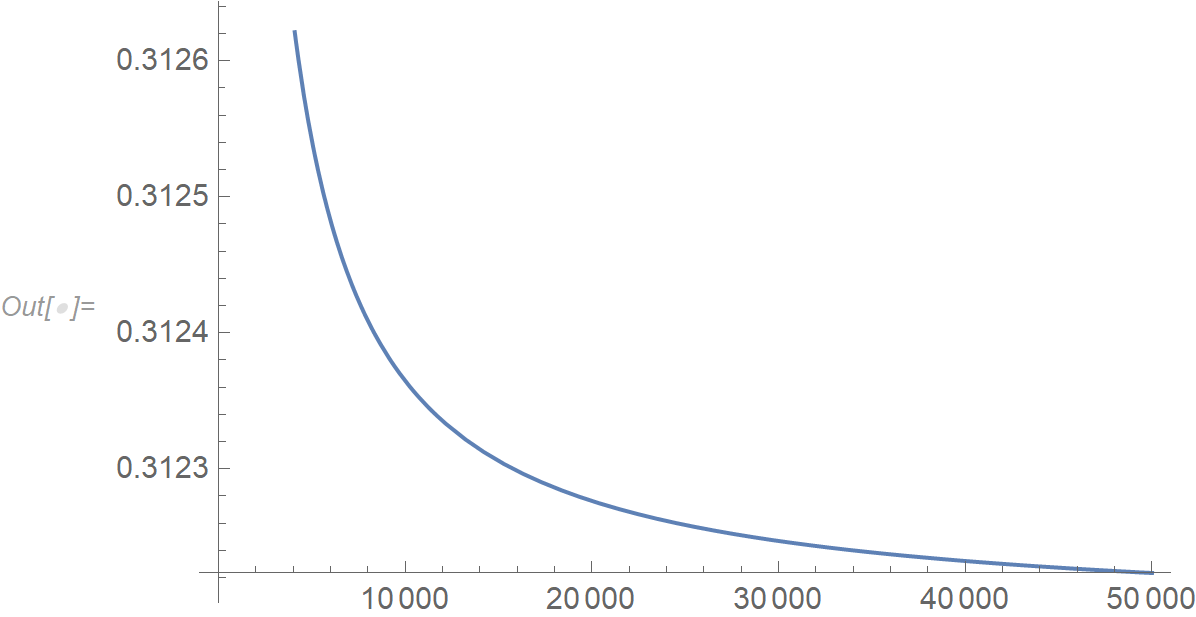
So we now have a solution for the minimum of the sum of squares given a value of c1. Plotting that minimum function against values of c1 shows that the absolute minimum is never realized for any finite value of c1:

Plot[sumOfSquares /. solc2, {c1, 0, 50000}]

Plot of sum of squares over values of c1

The limit of the sum of squares as c1 -> ∞ is

Limit[sumOfSquares /. solc2, c1 -> ∞] // N
(* 0.312188 *)

So any set of values with c2/.solc2 that has a sum of squares close to 0.312188 will give an almost identical fit.

Consider c1 = 4000. Then the values of c2 and the sum of squares are

solc2 /. c1 -> 4000 // N
(* {c2 -> 10569.9} *)

sumOfSquares /. solc2 /. c1 -> 4000 // N
(* 0.31263 *)

With c1 = 40000 we have

solc2 /. c1 -> 40000 // N
(* {c2 -> 105685.} *)

sumOfSquares /. solc2 /. c1 -> 40000 // N
(* 0.312232 *)

Finally: given the data that you have, just fitting a + b*log10q might be a better approach.

$\endgroup$
3
  • $\begingroup$ Thank you so much JimB for the nice explanation ! $\endgroup$
    – John
    Commented Jan 12, 2021 at 1:23
  • $\begingroup$ JimB one question: with the approach you show with the sum of squares close to 0.312, it is not very clear to me what would be the resulting values of C1 and C2. Could you clarify that if you don't mind. Thanks ! $\endgroup$
    – John
    Commented Jan 16, 2021 at 1:10
  • 1
    $\begingroup$ @John Added explicit examples for obtaining c2 given c1. $\endgroup$
    – JimB
    Commented Jan 16, 2021 at 6:15

Your Answer

By clicking “Post Your Answer”, you agree to our terms of service and acknowledge you have read our privacy policy.

Not the answer you're looking for? Browse other questions tagged or ask your own question.