2
$\begingroup$

I am trying to fit some data

data = {{100, 114}, {200, 1342}, {300, 36604}, {400, 44279}, {500, 
    10243}, {600, 4103}, {700, 3080}, {800, 2636}, {900, 2254}, {1000,
     1909}, {1100, 1821}, {1200, 1620}, {1300, 1436}, {1400, 
    1319}, {1500, 1175}, {1600, 1158}, {1700, 1094}, {1800, 
    975}, {1900, 884}, {2000, 865}, {2100, 806}, {2200, 721}, {2300, 
    630}, {2400, 634}, {2500, 650}, {2600, 530}, {2700, 498}, {2800, 
    465}, {2900, 462}, {3000, 400}, {3100, 442}, {3200, 376}, {3300, 
    364}, {3400, 362}, {3500, 305}, {3600, 292}, {3700, 313}, {3800, 
    292}, {3900, 240}, {4000, 243}, {4100, 281}, {4200, 230}, {4300, 
    231}, {4400, 229}, {4500, 227}, {4600, 208}, {4700, 215}, {4800, 
    182}, {4900, 176}, {5000, 191}, {5100, 187}, {5200, 177}, {5300, 
    170}, {5400, 170}, {5500, 157}, {5600, 135}, {5700, 120}, {5800, 
    154}, {5900, 162}, {6000, 118}, {6100, 131}, {6200, 116}, {6300, 
    142}, {6400, 142}, {6500, 157}, {6600, 135}, {6700, 151}, {6800, 
    172}, {6900, 128}, {7000, 126}, {7100, 117}, {7200, 113}, {7300, 
    127}, {7400, 120}, {7500, 114}, {7600, 132}, {7700, 133}, {7800, 
    140}, {7900, 107}, {8000, 135}, {8100, 163}, {8200, 117}, {8300, 
    118}, {8400, 103}, {8500, 111}, {8600, 107}, {8700, 126}, {8800, 
    89}, {8900, 109}, {9000, 107}, {9100, 127}, {9200, 101}, {9300, 
    101}, {9400, 107}, {9500, 116}, {9600, 111}, {9700, 109}, {9800, 
    110}, {9900, 111}, {10000, 97}, {10100, 88}, {10200, 107}, {10300,
     110}, {10400, 104}, {10500, 120}, {10600, 95}, {10700, 
    100}, {10800, 108}, {10900, 96}, {11000, 103}, {11100, 
    116}, {11200, 127}, {11300, 152}, {11400, 98}, {11500, 
    95}, {11600, 93}, {11700, 112}, {11800, 151}, {11900, 
    132}, {12000, 129}, {12100, 116}, {12200, 128}, {12300, 
    148}, {12400, 110}, {12500, 127}, {12600, 159}, {12700, 
    140}, {12800, 98}, {12900, 95}, {13000, 98}};
dataPlot = ListPlot[data, PlotRange -> All]

Plot of the list data

using a piecewise function consisting of a Gaussian function for $t < 600$ and an exponential function for $t \geq 600$. I've used FindFit and plotted the function on top of the data:

f2[t_, t0_, \[Sigma]_, t1_, \[Tau]_] := 
 Piecewise[{{A Exp[-((t - t0)/(Sqrt[2] \[Sigma]))^2], 
    t < 600}, {B Exp[-(t - t1)/\[Tau]], t >= 600}}]
FindFit[data, 
 f2[t, t0, \[Sigma], 
  t1, \[Tau]], {{t0, 400}, {\[Sigma], 100}, {t1, 600}, {\[Tau], 
   1000}, {A, 45000}, {B, 4000}}, t, 
 NormFunction -> (Norm[#1, Infinity] & )]
f2Fit[t_] := 
 Piecewise[{{45000*Exp[-((t - 360.003)/(Sqrt[2] 66.0556))^2], 
    t < 600}, {4000*Exp[-(t - 600)/1000], t >= 600}}]
fitPlot = 
  Plot[f2Fit[t], {t, 0, 13000}, PlotRange -> All, 
   PlotStyle -> {Red, Thick}];
Show[{dataPlot, fitPlot}]
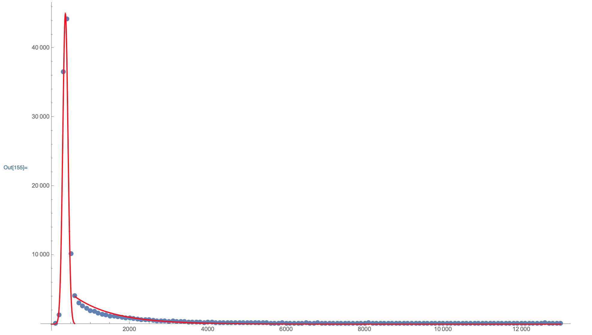
The fitted curve plotted on top of the data points but I am having some trouble getting the function to be continuous. I have tried tweaking parameters of the fit but this is very time consuming and doesn't work well. Is there a way I can force the FindFit function to generate a continuous piecewise function? Or is there another routine I can use to generate such a function?

$\endgroup$
2
  • $\begingroup$ I need the function to be continuous because I am trying to deconvolve it with another function and want to minimize as much noise as possible in the deconvolution. $\endgroup$ Commented Mar 30, 2020 at 19:48
  • $\begingroup$ If you want the function to be continuous (but not necessarily having the derivative to be continuous) at $t=600$, then you need to have $A \exp \left(-\left(\frac{t-\text{t0}}{\sqrt{2} \sigma }\right)^2\right)=B \exp \left(-\frac{t-\text{t1}}{\tau }\right)$ when $t=600$. That means there will be some restrictions among the parameters. Using Reduce on that equality suggests that using $\tau=-\frac{2 \sigma ^2 (t_1-600)}{2 \sigma ^2 \log \left(\frac{B}{A}\right)+t_0^2-1200 t_0+360000}$ would do it. $\endgroup$
    – JimB
    Commented Mar 30, 2020 at 20:13

1 Answer 1

4
$\begingroup$
Clear["Global`*"]

data = {{100, 114}, {200, 1342}, {300, 36604}, {400, 44279}, {500, 
    10243}, {600, 4103}, {700, 3080}, {800, 2636}, {900, 2254}, {1000, 
    1909}, {1100, 1821}, {1200, 1620}, {1300, 1436}, {1400, 1319}, {1500, 
    1175}, {1600, 1158}, {1700, 1094}, {1800, 975}, {1900, 884}, {2000, 
    865}, {2100, 806}, {2200, 721}, {2300, 630}, {2400, 634}, {2500, 
    650}, {2600, 530}, {2700, 498}, {2800, 465}, {2900, 462}, {3000, 
    400}, {3100, 442}, {3200, 376}, {3300, 364}, {3400, 362}, {3500, 
    305}, {3600, 292}, {3700, 313}, {3800, 292}, {3900, 240}, {4000, 
    243}, {4100, 281}, {4200, 230}, {4300, 231}, {4400, 229}, {4500, 
    227}, {4600, 208}, {4700, 215}, {4800, 182}, {4900, 176}, {5000, 
    191}, {5100, 187}, {5200, 177}, {5300, 170}, {5400, 170}, {5500, 
    157}, {5600, 135}, {5700, 120}, {5800, 154}, {5900, 162}, {6000, 
    118}, {6100, 131}, {6200, 116}, {6300, 142}, {6400, 142}, {6500, 
    157}, {6600, 135}, {6700, 151}, {6800, 172}, {6900, 128}, {7000, 
    126}, {7100, 117}, {7200, 113}, {7300, 127}, {7400, 120}, {7500, 
    114}, {7600, 132}, {7700, 133}, {7800, 140}, {7900, 107}, {8000, 
    135}, {8100, 163}, {8200, 117}, {8300, 118}, {8400, 103}, {8500, 
    111}, {8600, 107}, {8700, 126}, {8800, 89}, {8900, 109}, {9000, 
    107}, {9100, 127}, {9200, 101}, {9300, 101}, {9400, 107}, {9500, 
    116}, {9600, 111}, {9700, 109}, {9800, 110}, {9900, 111}, {10000, 
    97}, {10100, 88}, {10200, 107}, {10300, 110}, {10400, 104}, {10500, 
    120}, {10600, 95}, {10700, 100}, {10800, 108}, {10900, 96}, {11000, 
    103}, {11100, 116}, {11200, 127}, {11300, 152}, {11400, 98}, {11500, 
    95}, {11600, 93}, {11700, 112}, {11800, 151}, {11900, 132}, {12000, 
    129}, {12100, 116}, {12200, 128}, {12300, 148}, {12400, 110}, {12500, 
    127}, {12600, 159}, {12700, 140}, {12800, 98}, {12900, 95}, {13000, 98}};

{tmin, tmax} = MinMax@data[[All, 1]];

Use NonlinearModelFit, make the transition value a parameter, and include a constraint for continuity at the transition value.

f2[t_, t0_, σ_, t1_, τ_, trans_] := 
 Piecewise[{{A Exp[-((t - t0)/(Sqrt[2] σ))^2], 
    t < trans}, {B Exp[-(t - t1)/τ], t >= trans}}]

(nlm = NonlinearModelFit[data, {f2[t, t0, σ, t1, τ, trans],
     A Exp[-((trans - t0)/(Sqrt[2] σ))^2] == 
      B Exp[-(trans - t1)/τ]},
    {{t0, 400}, {σ, 100}, {t1, 600}, {τ, 1000}, {A, 45000}, {B, 
      4000}, {trans, 600}}, t]) // Normal

enter image description here

Plot[nlm[t], {t, tmin, tmax},
 PlotStyle -> Red,
 PlotPoints -> 100,
 MaxRecursion -> 5,
 PlotRange -> All,
 Epilog -> {Inset[
    Plot[nlm[t], {t, 520, 560},
     PlotStyle -> Red,
     PlotPoints -> 100,
     MaxRecursion -> 5,
     PlotLabel -> "model is continuous"]],
   AbsolutePointSize[2], Point[data]}]

enter image description here

nlm["Properties"]

{"AdjustedRSquared", "AIC", "AICc", "ANOVATable", \
"ANOVATableDegreesOfFreedom", "ANOVATableEntries", \
"ANOVATableMeanSquares", "ANOVATableSumsOfSquares", "BestFit", \
"BestFitParameters", "BIC", "CorrelationMatrix", "CovarianceMatrix", \
"CurvatureConfidenceRegion", "Data", "EstimatedVariance", \
"FitCurvatureTable", "FitCurvatureTableEntries", "FitResiduals", \
"Function", "HatDiagonal", "MaxIntrinsicCurvature", \
"MaxParameterEffectsCurvature", "MeanPredictionBands", \
"MeanPredictionConfidenceIntervals", \
"MeanPredictionConfidenceIntervalTable", \
"MeanPredictionConfidenceIntervalTableEntries", \
"MeanPredictionErrors", "ParameterBias", \
"ParameterConfidenceIntervals", "ParameterConfidenceIntervalTable", \
"ParameterConfidenceIntervalTableEntries", \
"ParameterConfidenceRegion", "ParameterErrors", "ParameterPValues", \
"ParameterTable", "ParameterTableEntries", "ParameterTStatistics", \
"PredictedResponse", "Properties", "Response", "RSquared", \
"SingleDeletionVariances", "SinglePredictionBands", \
"SinglePredictionConfidenceIntervals", \
"SinglePredictionConfidenceIntervalTable", \
"SinglePredictionConfidenceIntervalTableEntries", \
"SinglePredictionErrors", "StandardizedResiduals", \
"StudentizedResiduals"}
$\endgroup$
2
  • $\begingroup$ Thank you so much! I didn't think to set the transition value as a fit parameter but that seems like an obvious solution now. What are the differences between NonlinearModelFit and FindFit? $\endgroup$ Commented Mar 30, 2020 at 21:45
  • $\begingroup$ NonlinearModelFit has many properties and diagnostics. See the documentation. $\endgroup$
    – Bob Hanlon
    Commented Mar 30, 2020 at 21:54

Your Answer

By clicking “Post Your Answer”, you agree to our terms of service and acknowledge you have read our privacy policy.

Not the answer you're looking for? Browse other questions tagged or ask your own question.