9
$\begingroup$

I have a 3×3 error covariance in Mathematica, but I don't know how to use it for plotting the error ellipsoid. It would be great if you can show me how I can do that for the below covariance matrix:

CovMat= {{88.5333, -33.6, -5.33333}, 
         {-33.6, 15.4424, 2.66667}, 
         {-5.33333, 2.66667, 0.484848}}

eigenvalues= {0.0098, 0.4046, 104.7}

eigenvectors= {{0.93, 0.36, -0.03}, {-0.36, 0.9, -0.23}, {-0.06, 0.23, 0.97}}

And as the last question, how can I project this ellipsoid onto 2D planes?

$\endgroup$
0

3 Answers 3

12
$\begingroup$

For full control over the plot and the analysis, it is useful to know how to do the calculations yourself. They include:

  • Finding the contour level corresponding to the desired confidence (without this the result scarcely can be called a "confidence" ellipse!);

  • Determining the limits (and aspect ratios) of the plot;

  • Establishing a useful mesh on the ellipsoid (showing contours along the eigendirections).

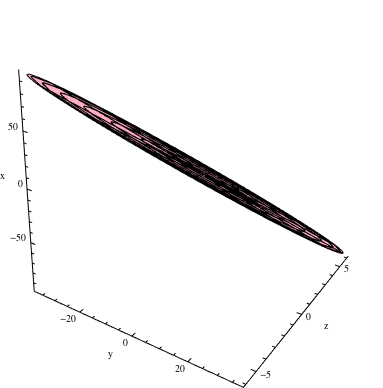
These steps should be apparent in the lines of the following code, which takes for input a number a (the confidence will be $1-a$) and the covariance matrix, here called c:

limit[ci_, n_, t_] := Abs[n.{x, y, z}] /. 
  Last[NMaximize[{(n.{x, y, z})^2, {x, y, z}.ci.{x, y, z} <= t}, {x, y, z}]];
Block[{t = InverseCDF[ChiSquareDistribution[3], 1 - 0.05], ci = Inverse[c], x0, y0, z0, mf},
 {x0, y0, z0} = 1.05 limit[ci, #, t] & /@ IdentityMatrix[3];
 mf = Function[{x, y, z}, #.{x, y, z}] & /@ Eigenvectors[c];
 ContourPlot3D[{x, y, z}.ci.{x, y, z} == t, {x, -x0, x0}, {y, -y0, y0}, {z, -z0, z0}, 
  AxesLabel -> {x, y, z}, 
  ContourStyle -> Opacity[0.8],
  MeshFunctions -> mf , MeshStyle -> Opacity[0.2], 
  BoxRatios -> {x0, y0, z0}]]

limit finds the extreme absolute values of any linear form (given by a three-vector n) along the ellipse specified by matrix ci at level t. You can observe its use within the subsequent Block where, by applying it to the three vectors $(1,0,0)$, $(0,1,0)$, and $(0,0,1)$ (the rows of IdentityMatrix), we obtain the extreme values of $x$, $y$, and $z$ in the plot (and expand them by five percent to give a small margin).

mf computes the distances along the eigenvectors.

InverseCDF computes the proper contour level for the desired confidence.

Note that the confidence ellipsoid is a contour of the inverse of the covariance matrix.
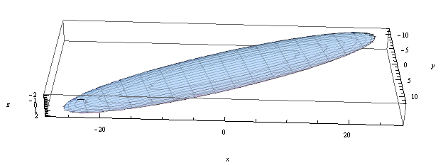
Figure


In another answer, @rm-rf has given some expedient ways to plot projections. You can also use the technique given above to draw slices through the ellipsoid: simply fix one of $x$, $y$, or $z$ (perhaps by making it controllable by Manipulate) and invoke ContourPlot instead of ContourPlot3D, changing the arguments in obvious ways. This would be a nice way to obtain conditional confidence ellipses.

$\endgroup$
8
  • $\begingroup$ Thank you for suggesting a more flexible way of plotting this ellipsoid. The only part I cannot fully understand is the "Level t". What does it do exactly? $\endgroup$
    – K-1
    Commented Mar 18, 2013 at 1:31
  • $\begingroup$ @K-1 There are infinitely many confidence ellipses ("error ellipsoids"), each determined by its corresponding "confidence level," a number between $0$ and $1$. That's what t is based on: you can see its calculation at the beginning of the Block. $\endgroup$
    – whuber
    Commented Apr 8, 2013 at 15:49
  • 2
    $\begingroup$ NMaxValue[] would allow for a more compact implementation of limit[]. $\endgroup$ Commented Apr 11, 2013 at 10:35
  • 1
    $\begingroup$ @Vladimir I appreciate your nuance, but something's missing: you still haven't even stated what your interpretation is! That is, for what purposes would one "do marginalization"? Until you're explicit and forthcoming about that, I don't see how your remark could help beginners. It seems to me that the only clear message it conveys is "Bad! Don't pay attention to this answer! Read my question instead!" $\endgroup$
    – whuber
    Commented Apr 19, 2013 at 20:54
  • 1
    $\begingroup$ hahaha No, no, sorry, that's not what I wanted to say! I was more explicit to drag attention, only because comments are not often read. Honestly, I myself learned a lot from this answer and it is actually the answers for my question, too! (which is why I called it brilliant, as it is for any dimension). And now: if you are not interested in one variable and you want to see confidence regions for the rest of variables, you can either put some fixed value to that one variable and get new correlation matrix (by fitting again), or integrate probability function over that variable, eg. marginalize. $\endgroup$
    – Vladimir
    Commented Apr 19, 2013 at 21:42
8
$\begingroup$

Ellipsoids can be easily plotted using the MultivariateStatistics` package. The eigenvalues of your covariance matrix denote the lengths of the axes and the eigenvectors, their orientation. Here's how it can be done for your CovMat:

CovMat = {{88.5333, -33.6, -5.33333}, 
          {-33.6, 15.4424, 2.66667}, 
          {-5.33333, 2.66667, 0.484848}};

e = Ellipsoid[{0, 0, 0}, Sequence @@ Eigensystem[CovMat]];
Graphics3D[e, BoxRatios -> 1, Axes -> True, Boxed -> False, AxesLabel -> {"x", "y", "z"}]

You can get the different projections by altering the ViewPoint:

Graphics3D[e, BoxRatios -> 1, Axes -> True, Boxed -> False, 
    AxesLabel -> {"x", "y", "z"}, ViewPoint -> #, 
    ImageSize -> 200] & /@ Permutations[{0, 0, Infinity}, {3}] // Row[#, Spacer[10]] &

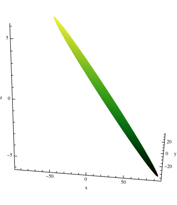
If you want better control over the appearance of your ellipsoid, you should do the plotting yourself with ParametricPlot3D (which is what Ellipsoid does behind the scenes). For example:

ParametricPlot3D[
   Transpose[#2].(# {Cos[t] Cos[u], Sin[t] Cos[u], Sin[u]}), {t, 0, 2 π}, {u, -(π/2), π/2}, 
    Boxed -> False, BoxRatios -> 1, AxesLabel -> {"x", "y", "z"}, 
   ColorFunction -> "AvocadoColors", Mesh -> False] & @@ Eigensystem@CovMat

$\endgroup$
1
  • $\begingroup$ Thank you rm-rf for your answer. It was quite helpful! $\endgroup$
    – K-1
    Commented Mar 18, 2013 at 1:30
5
$\begingroup$

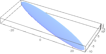
Since Ellipsoid[] is now built-in, and has a different syntax from the version that was once in MultivariateStatistics`​, let me present the way to render the confidence ellipsoid corresponding to a given covariance matrix:

c = {{88.5333, -33.6, -5.33333}, 
     {-33.6, 15.4424, 2.66667}, 
     {-5.33333, 2.66667, 0.484848}};

With[{α = 0.05}, (* level of significance *)
     ell = Ellipsoid[{0, 0, 0}, InverseCDF[ChiSquareDistribution[3], 1 - α] c]];

Graphics3D[ell, Axes -> True]

confidence ellipsoid

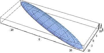
If you want to render the ellipsoid's contours along its eigendirections, you can do this:

vecs = Eigenvectors[c];

RegionPlot3D[ell, Axes -> True, AxesStyle -> Opacity[1, Black], BaseStyle -> Transparent,
             Mesh -> 10, MeshFunctions -> Evaluate[Map[Function, vecs.{#1, #2, #3}]], 
             MeshStyle -> Opacity[1, Black], PlotStyle -> Opacity[1, White], 
             TicksStyle -> Opacity[1, Black]]

eigencontours

where some of the option settings (e.g. BaseStyle -> Transparent) was needed to work around a bug in RegionPlot3D[] involving meshline rendering.

$\endgroup$

Your Answer

By clicking “Post Your Answer”, you agree to our terms of service and acknowledge you have read our privacy policy.

Not the answer you're looking for? Browse other questions tagged or ask your own question.