3
$\begingroup$

If I have a list of points in 3D space that are only roughly located on a surface, this surface can be visualized with ListSurfacePlot3D. How can I find the intersection of this approximate surface with a plane, that spans between two vectors u and v? And to continue this, how would I find the intersection of the resulting line with another plane that spans between two vectors m and n?

The dataset of points is available here: https://www.dropbox.com/s/rlj91jrh1bp4g2c/data.txt?dl=0

$\endgroup$
1
  • $\begingroup$ Crossposted here. $\endgroup$ Commented Sep 24, 2019 at 16:23

2 Answers 2

3
$\begingroup$

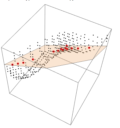
Being the dataset in the form of a number of points on a surface, it is not a trivial problem to compute the intersection between such a surface and a plane.

One way can be to find the sets of points on the surface that are closer to the given plane more than a preset threshold. Here is a way to do this (note that I am not using ListSurfacePlot3D at all here):

distancePointFromPlane[point_, planeV1_, planeV2_, 
   planeTranslation_] := 
  With[{orthogonalVec = #/Norm@# &@Cross[planeV1, planeV2]},
   Norm@Dot[orthogonalVec, point - planeTranslation]
   ];
distancePointsFromPlane[points_, planeV1_, planeV2_, 
   planeTranslation_] := 
  With[{orthogonalVec = #/Norm@# &@Cross[planeV1, planeV2]},
   Norm@Dot[orthogonalVec, # - planeTranslation] & /@ points
   ];
findPointsCloseToPlane[points_, planeV1_, planeV2_, planeTranslation_,
    maxDistance_] := Thread@{
      Range@Length@points,
      distancePointsFromPlane[points, planeV1, planeV2, 
       planeTranslation]
      } // Select[#, #[[2]] <= maxDistance &] & // Map@First;

planeV1 = {1, 1, 0};
planeV2 = {1, -1, 1};
planeTranslation = {0, 0, 0.7};
dataPoints = 
  Import["./data.txt"] // StringReplace[#, "\n" -> ""] & // 
   ToExpression;
With[{pts = dataPoints},
 Graphics3D[{
   {Red, [email protected], Point@pts[[
      findPointsCloseToPlane[pts, planeV1, planeV2, planeTranslation, 
       0.01]
      ]]},
   Point@pts,
   [email protected], InfinitePlane[planeTranslation, {planeV1, planeV2}]
   }]
 ]
Graphics3D[{Point@dataPoints}]

enter image description here

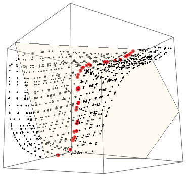
The results are not great though. You will get better results if the points of the surface are denser. A quick and dirty way to do this is to use ListSurfacePlot3D to build an interpolating surface, and then retrieve the points from the generated graphics:

planeV1 = {1, 1, 0};
planeV2 = {1, -1, 1};
planeTranslation = {0, 0, 0.7};
dataPoints = 
  Import["./data.txt"] // StringReplace[#, "\n" -> ""] & // 
   ToExpression;
With[{pts = ListSurfacePlot3D[dataPoints][[1, 1]]},
 With[{goodPoints = 
    findPointsCloseToPlane[pts, planeV1, planeV2, planeTranslation, 
     0.01]},
  Graphics3D[{
    {Red, [email protected], Point@pts[[goodPoints]]},
    Point@pts,
    [email protected], InfinitePlane[planeTranslation, {planeV1, planeV2}]
    }]
  ]]

enter image description here

There is still plenty of room to improve, but it already looks much better I think.

$\endgroup$
2
  • $\begingroup$ that's not too bad.. what would be a less dirty way to increase the density of the points even more? Or can I iteratively feed the points from ListSurfacePlot3D to a new ListSurfacePlot3D and get an even denser set of points? $\endgroup$
    – piiipmatz
    Commented Sep 24, 2019 at 22:06
  • $\begingroup$ @piiipmatz you could try playing with the value of the MaxPlotPoints option of ListSurfacePlot3D. $\endgroup$
    – glS
    Commented Sep 26, 2019 at 16:00
3
$\begingroup$

Update: Using MeshFunctions to get the intersection of the plane and ListSurfacePlot3D surface:

We can use the points p1, v1 and v2 to get the equation of the plane ip:

Simplify[Cross[v1, v2].({x, y, z} - p1)]

7/5 + x - y - 2 z

and use it as the MeshFunctions option value to show the intersection of ListSurfacePlot3D and ip:

lsp = ListSurfacePlot3D[data, Axes -> False, 
    MeshFunctions -> {7/5 + # - #2 - 2 #3  &}, Mesh -> {{0.}}, 
    MeshStyle -> Directive[Red, Thick], 
    MeshShading -> {Opacity[.5, Yellow], Opacity[.5, Blue]},  
    BoxRatios -> 1];

Show[lsp, Graphics3D[{Lighting -> "Neutral", Point @ data,
     Red, Sphere[#, .01] & /@ pts, EdgeForm[], Opacity[.3, Green], ip}]]
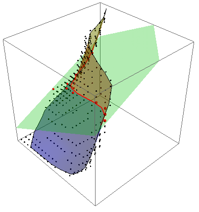
enter image description here

We can do the same for arbitrary function f that defines a plane through f == 0. For example,

f[x_, y_, z_, w_]:= x - y + 2 z - w; (* the plane x - y + 2 z  == w *)

Show[ListSurfacePlot3D[data, 
    Axes -> False, 
    MeshFunctions -> {f[#, #2, #3, 1] &}, Mesh -> {{0}}, 
    MeshStyle -> Directive[Red, Thick], 
    MeshShading -> {Opacity[.5, Blue], Opacity[.5, Yellow]}, 
    BoxRatios -> 1, BoundaryStyle -> None], 
  ListPointPlot3D[data], 
  ContourPlot3D[f[x, y, z, 1] == 0, {x, 0, 1}, {y, 0, 1}, {z, 0, 1} , 
   BoundaryStyle -> None, 
   ContourStyle -> Opacity[.25, Purple], 
   Mesh -> None]]
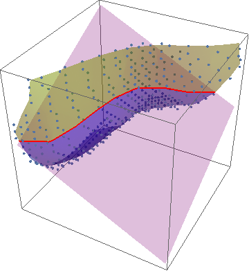
enter image description here

Original answer:

Using the same InfinitePlane as in glS's answer:

p1 = {0, 0, 7/10};
v1 = {1, 1, 0};
v2 = {1, -1, 1};
dist = .01;

ip = InfinitePlane[p1, {v1, v2}];

Points within dist of ip can be obtained using Select and RegionDistance:

pts = Select[data, RegionDistance[ip, #] <= dist &];

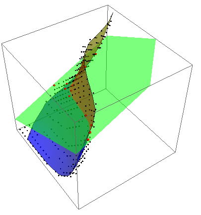
We can also use ip as the value for ClippingPlanes directive to style parts of the surface above and below the plane differently:

lsp = ListSurfacePlot3D[data, Axes -> False, 
    Mesh -> None, PlotStyle -> Opacity[.7, Yellow],  BoxRatios -> 1];

Graphics3D[{Lighting -> "Neutral", Point @ data,
  Red, Sphere[#, .01] & /@ pts, lsp[[1]], 
  ClipPlanes -> ip, ClipPlanesStyle -> Opacity[.3, Green], 
  Opacity[.7, Blue], lsp[[1]] /. Directive[__] :> {}}]
enter image description here

$\endgroup$
5
  • $\begingroup$ How does Graphics3D determine the parts above and below? This must include determining the line at the intersection of the green plane with the surface that is interpolated from the points? $\endgroup$
    – piiipmatz
    Commented Sep 24, 2019 at 13:59
  • $\begingroup$ @piiipmatz, ClipPlanes >> Details says "ClipPlanes -> {{a1,b1,c1,d1}, {a2,b2,c2,d2},...} specifies a list of clipping planes defined as ai x + bi y + ci z + di <=0" $\endgroup$
    – kglr
    Commented Sep 24, 2019 at 14:30
  • $\begingroup$ my question was more related to the actual algorithm behind the scene! I.e. it is nice if the plot function can do all that stuff, but what if I wanted to use the intersection for further calculations? Using MeshFunctions you get this very nice red curve in the plot but what are the coordinates of the points on this curve? $\endgroup$
    – piiipmatz
    Commented Sep 24, 2019 at 21:56
  • $\begingroup$ @piiipmatz, if you have the patience/perserverence you can inspect the output of ClearAttributes[Region`InfinitePlaneCuboidClip, {Protected, ReadProtected}]; Graphics3D[{Sphere[]}, ClipPlanes -> InfinitePlane[{{0, 0, 0}, {0, 1, 1}, {1, 1, 2}}]]; ??Region`InfinitePlaneCuboidClip for an example of what goes on "behind the scene". $\endgroup$
    – kglr
    Commented Sep 24, 2019 at 22:19
  • $\begingroup$ @piiipmatz, re "what are the coordinates of the points on this curve", you can try lsp=ListSurfacePlot3D[data, Axes -> False, MeshFunctions -> {f[#, #2, #3, 1] &}, Mesh -> {{0}}, MeshStyle -> Directive[Red, Thick], MeshShading -> {Opacity[.5, Blue], Opacity[.5, Yellow]}, BoxRatios -> 1, BoundaryStyle -> None]; pointsoncurve=Cases[Normal[lsp], Line[x]:>x, All]. $\endgroup$
    – kglr
    Commented Sep 24, 2019 at 22:21

Your Answer

By clicking “Post Your Answer”, you agree to our terms of service and acknowledge you have read our privacy policy.

Not the answer you're looking for? Browse other questions tagged or ask your own question.