10
$\begingroup$

I'm not super familiar with Principal Component Analysis, but from what I understand, it sorts a vector in order of decreasing variance, and uses that to transform the vector to correlate variables linearly.

I'm not trying to transform the data I have - I'm simply trying, for a list of 784-length feature vectors, to get the PCA "scores" for each feature. Mathematica returns them sorted - I need to be able to correlate them with the actual features, so I need them in their original order. PrincipalComponents doesn't seem to be able to return anything in this format. Is there a way to?

$\endgroup$
2
  • 2
    $\begingroup$ does PrincipalComponents[data][[Ordering @ data]] or PrincipalComponents[data][[Ordering[Variance/@ data]]] give what you need? $\endgroup$
    – kglr
    Commented Aug 9, 2019 at 15:36
  • $\begingroup$ @kglr Since I'm passing PrincipalComponents a 10x784 matrix, that seems to just reorder the 784-length sublists, rather than the values within those lists. I want to correlate the PCA scores with the feature (value in the 784-length list) they actually correspond to. $\endgroup$
    – Nico A
    Commented Aug 9, 2019 at 15:38

1 Answer 1

13
$\begingroup$

You're in luck, because I recently waded through this problem myself. If I understand your question correctly, you want to know the matrix that transforms the data into the output of PrincipalComponents. The answer to this: that matrix is just the eigenvectors of the correlation matrix.

Simple 2D example:

data = RandomVariate[BinormalDistribution[{-1, 2}, {1, 2}, 0.9], 100];
eig = Eigensystem[Covariance[data]];
ListPlot[
 {
  PrincipalComponents[data],
  Standardize[data, Mean, 1 &].Transpose[eig[[2]]]
  }
 ]
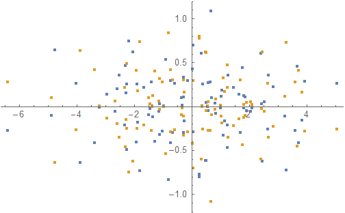
plot

As you can see, the result is the same, except for the two clouds being mirrored in the x-axis. This makes sense, since principal component analysis is about transforming the data such that the covariance matrix becomes diagonal (with the diagonal decreasing towards the bottom right) and flipping the data along an axis leaves the covariance invariant.

As a bonus, the eigenvalues of the covariance matrix tell you how much variance each principal component accounts for, so you don't have to calculate that separately:

eig[[1]]
Variance[PrincipalComponents[data]]

Out[142]= {4.62687, 0.137012}

Out[143]= {4.62687, 0.137012}

edit: You can also reproduce the principle components using SingularValueDecomposition. See the following answer by J.M.

$\endgroup$
2
  • $\begingroup$ I am personally more inclined to use SVD rather than the eigendecomposition for this. Using the equivalences presented here, we have the identity PrincipalComponents[data] == Apply[Dot, Most[SingularValueDecomposition[Standardize[data, Mean, 1 &]]]]. Additionally, Eigenvectors[Covariance[data]] is just the same as Last[SingularValueDecomposition[Standardize[data, Mean, 1 &]]] (modulo changes in signs). $\endgroup$ Commented Aug 12, 2019 at 9:29
  • 1
    $\begingroup$ Yes, that is another possibility I ran into. Is there a good reason to prefer SVD for this? I found that computing the eigenvectors of the covariance matrix is generally faster for large datasets than computing the (truncated) SVD. Are there other numerical reasons for preferring one over the other? In addition: the covariance matrix is often a quantity of interest anyway, so if you're going to compute that, you might as well use it for the principle components too (since it's just a small step from there). That's my reasoning, at least. $\endgroup$ Commented Aug 12, 2019 at 10:18

Your Answer

By clicking “Post Your Answer”, you agree to our terms of service and acknowledge you have read our privacy policy.

Not the answer you're looking for? Browse other questions tagged or ask your own question.