Using NDEigensystem to solve the Mathieu equation

Question

To be able to apply the differential equation capabilities of Mathematica to my graduate thesis, I am trying to apply NDEigensystem to an eigenproblem whose solution I know, but I am having some trouble doing so.

As a test problem, I am using an algebraic version of the Mathieu equation,

$$(1-\zeta^{2})w^{\prime\prime}-\zeta w^{\prime}+\left(a+2q-4q\zeta^{2}\right)w=0$$

For this example I set $q=4/3$ and take only the first three eigenpairs:

m = 3; q = 4/3;
op = -(1 - ζ^2) u''[ζ] + ζ u'[ζ] + 2 q (2 ζ^2 - 1) u[ζ];
bc = DirichletCondition[u[ζ] == 0, True];
{λ, fl} = NDEigensystem[{op, bc}, u, {ζ, 0, 1}, m];

I chose the Mathieu equation as a nontrivial example as Mathematica already has a function for its evaluation:

λt = Table[MathieuCharacteristicB[2 k, q], {k, m}];
flt = Table[With[{k = k, q = q},
MathieuS[MathieuCharacteristicB[2 k, q], q, ArcCos[#]] &], {k, m}];

The problem is, I do not get the expected eigenvalues!

λ
(* {4.0708, 17.3259, 39.1877} *)
N[λt]
(* {3.85298, 16.0581, 36.0254} *)

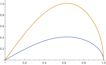
And of course, plotting shows that the eigenequation is not satisfied at all:

With[{u = fl[[1]], b = λ[[1]]},
     Plot[(1 - ζ^2) u''[ζ] - ζ u'[ζ] + (b + 2 q - 4 q ζ^2) u[ζ], {ζ, 0, 1}]]
With[{u = flt[[1]], b = λt[[1]]},
     Plot[(1 - ζ^2) u''[ζ] - ζ u'[ζ] + (b + 2 q - 4 q ζ^2) u[ζ], {ζ, 0, 1}]]

What was wrong with my attempt? If I can get this example to work, I should be able to apply it to my actual, more complicated problem, so any good ideas would be welcome.

Answer 1

It looks to me like NDEigensystem is struggling with the singularity at $\zeta=1$, as does the method that I'm going to show. But perhaps it'll be useful for you, at least as a cross-check.

I have a package for numerically calculating solutions of eigenvalue problems using the Evans function via the method of compound matrices, which is hosted on github. See my answers to other questions, the example notebook on the github or this introduction for some more details.

First we install the package (only need to do this the first time):

Needs["PacletManager`"]
PacletInstall["CompoundMatrixMethod", 
    "Site" -> "http://raw.githubusercontent.com/paclets/Repository/master"]

Then we first need to turn the ODEs into a matrix form $\mathbf{y}'=\mathbf{A} \cdot \mathbf{y}$, using my function ToMatrixSystem:

Needs["CompoundMatrixMethod`"]
m = 3; q = 4/3;
op = -(1 - ζ^2) u''[ζ] + ζ u'[ζ] + 2 q (2 ζ^2 - 1) u[ζ];
sys[ζend_] = ToMatrixSystem[op == a u[ζ], {u[0] == 0, u[ζend] == 0}, u, {ζ, 0, ζend}, a]

Now the function Evans will calculate the Evans function (also known as the Miss-Distance function) for any given value of $a$ and $\zeta_{end}$; this is an analytic function whose roots coincide with eigenvalues of the original equation.

Plugging in $\zeta_{end} = 1$ fails due to the singularity, but you can try moving the endpoint slightly away:

FindRoot[Evans[a, sys[1 - 10^-3]], {a, 3}]
(* {a -> 4.00335} *)

Moving the endpoint closer approaches the correct value, but I can't get the exact value with this method.

aEvans = a /. FindRoot[Evans[a, sys[1 - 10^-10], WorkingPrecision -> 30], {a, 3}, 
  WorkingPrecision -> 30] // Quiet
(* {a -> 3.85301} *)

My package can't get the eigenfunctions directly at the moment, but you can use this eigenvalue in NDSolve (with an arbitrary second condition at $\zeta=0$, set it to be 2.45446 to make it consistent with the MathieuS):

sol = NDSolveValue[{op == aEvans u[\[Zeta]], {u[0] == 0, u'[0] == 1}},
   u, {\[Zeta], 0, 1 - 10^-10}];
Plot[{sol[\[Zeta]], flt[[1]][\[Zeta]]}, {\[Zeta], 0, 1 - 10^-10}]

The same should work for the other roots.

Answer 2

If you refine the mesh, you will get closer:

m = 3; q = 4/3;
op = -(1 - \[Zeta]^2) u''[\[Zeta]] + \[Zeta] u'[\[Zeta]] + 
   2 q (2 \[Zeta]^2 - 1) u[\[Zeta]];
bc = DirichletCondition[u[\[Zeta]] == 0, True];
{\[Lambda], fl} = 
  NDEigensystem[{op, bc}, u, {\[Zeta], 0, 1}, m, 
   Method -> {"PDEDiscretization" -> {"FiniteElement", {"MeshOptions" \
-> {"MaxCellMeasure" -> 0.00001}}}}];

\[Lambda]
{3.855, 16.074, 36.064}

\[Lambda]t = Table[MathieuCharacteristicB[2 k, q], {k, m}];
flt = Table[
   With[{j = j}, 
    MathieuS[MathieuCharacteristicB[2 k, q], q, ArcCos[#]] &], {k, m}];

\[Lambda]t // N
{3.852, 16.058, 36.025}