2
$\begingroup$

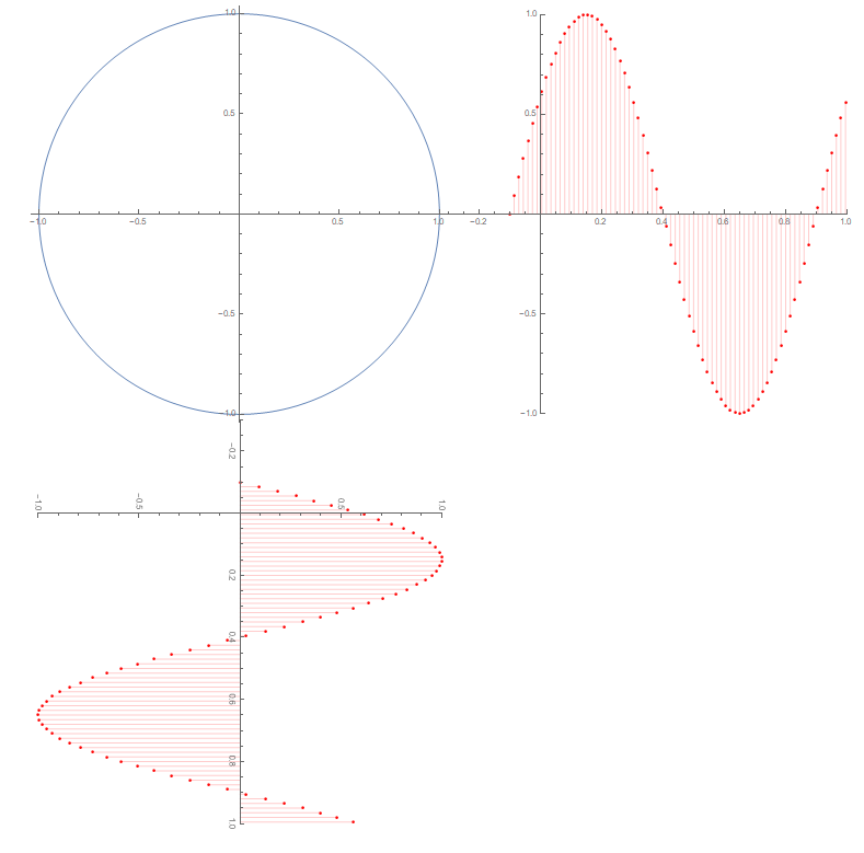
I want to plot an orthographic (as in "drafting" with top, side, and front view) of a complex sinusoid in time. Here's my attempt:

a = -0.1
b = 1.0
\[Nu] = 1.0
\[Eta] = .1*2*\[Pi]
A = 1.0
f[t_] := A*Sin[2*\[Pi]*\[Nu]*t + \[Eta]]
p1 := PolarPlot[A, {t, 0, 2 \[Pi]}]
p2 := DiscretePlot[f[t], {t, a, b, 0.015}, PlotStyle -> Red]
p3 := Rotate[p2, 3 \[Pi]/2]
GraphicsGrid[{{p1, p2}, {p3}}]

But, the 3 views have different scale factors. Is there a way to require a common scale, or is there a better approach? Thx, Dave

$\endgroup$
3
  • $\begingroup$ Try adding AspectRatio -> Automatic to p2. $\endgroup$
    – MelaGo
    Commented Apr 10, 2019 at 1:08
  • $\begingroup$ Thanks! AspectRatio->Automatic worked well. However, when I change image size either by click & drag or Show ImageSize->Large, the rotated plot doesn't change size. Any idea why and how to control its scale? $\endgroup$ Commented Apr 10, 2019 at 18:23
  • $\begingroup$ On closer look, AspectRatio->Automatic "almost" did the trick. What I want is the ability to make the axes of 2 different plot on the same graphic to be the same length: I want control over scale, position, and rotation of 3 plots in the same graphic. Thanks... $\endgroup$ Commented Apr 10, 2019 at 18:57

2 Answers 2

2
$\begingroup$

How about this:

a = -0.1;
b = 1.0;
\[Nu] = 1.0;
\[Eta] = .1*2*\[Pi];
A = 1.0;
f[t_] := A*Sin[2*\[Pi]*\[Nu]*t + \[Eta]];
p2 = DiscretePlot[f[t], {t, a, b, 0.015}, PlotStyle -> Red, 
   AspectRatio -> Automatic, PlotRange -> {{-.2, 1}, {-1, 1}}];

PolarPlot[A, {t, 0, 2 \[Pi]}, 
 Ticks -> {Range[-1, 1, .2], Range[-1, 1, .2]},
 Epilog -> {Inset[p2, {1.4, 0}, {0, 0}, Scaled[{1, .5}]],
   Inset[p2, {0, -1.4}, {0, 0}, Scaled[{1, .5}], {0, -1}]},
 PlotRange -> {{-1.5, 2.5}, {-2.5, 1.5}}]

enter image description here

$\endgroup$
3
  • $\begingroup$ I feel this is overly "tricky" to get everything on the same axes. It might be better to do it somehow with Show, but I haven't figured it out. $\endgroup$
    – MelaGo
    Commented Apr 10, 2019 at 22:00
  • $\begingroup$ Thanks MelaGo, I $\endgroup$ Commented Apr 11, 2019 at 19:29
  • $\begingroup$ ... I agree it seems like there should be a "Show" approach. I'll keep an eye open for it... $\endgroup$ Commented Apr 11, 2019 at 19:38
2
$\begingroup$

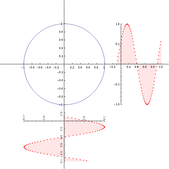
There must be a more natural way to have common scales but here is one way that requires the tweaking of the ImageSize values. The main "fix" to get the figures to line up is to use a negative Spacings in GraphicsGrid.

a = -0.1
b = 1.0
ν = 1.0
η = .1*2*π
A = 1.0
f[t_] := A*Sin[2*π*ν*t + η]
p1 = PolarPlot[A, {t, 0, 2 π}, AspectRatio -> 1, ImageSize -> 510];
p2 = DiscretePlot[f[t], {t, a, b, 0.015}, PlotStyle -> Red, 
   AspectRatio -> 1, PlotRange -> {{-0.3, 1}, {-1, 1}}, ImageSize -> 500];
p3 = Rotate[p2, 3 π/2];
GraphicsGrid[{{p1, p2}, {p3}}, Spacings -> -10]

Plots at same scale

When the ImageSize is chosen to be the same for both p1 and p2, then the plots don't quite line up properly. Using 510 and 500 (or 305 and 300) seems have the plots line up reasonably.

$\endgroup$
1
  • $\begingroup$ Yes, thanks JimB, for the benefit of your insight. I'm disappointed there's not a more natural way to do this, but at least I can achieve my objective. $\endgroup$ Commented Apr 11, 2019 at 19:29

Your Answer

By clicking “Post Your Answer”, you agree to our terms of service and acknowledge you have read our privacy policy.

Not the answer you're looking for? Browse other questions tagged or ask your own question.