I am trying to fit the following tide data (taken from here) with a sinusoidal curve that looks like the following: displacement+amplitude * sin(t w - ph), where t is the independent variable, w is the angular frequency, ph is the phase, displacement is the average offset from zero, and amplitude is the sine curve's amplitude.
(* Times measured from midnight, 28 September (hours) *)
xd = {19.4000, 25.6333, 31.7833, 38., 44.1167, 50.3667, 56.4667,
   62.6833, 68.8167, 75.0500, 81.1333, 87.3333, 93.5000, 99.7500,
   105.8000, 112.0167};
(* Tidal heights offset from standard water level (m) *)
yd = {0.88, 12.71, 0.88, 12.63, 0.78, 12.59, 1.06, 12.57, 0.88, 12.32,
    1.40, 12.35, 1.15, 11.94, 1.84, 12.02};
samples = Transpose[{xd, yd}];
Thus far, I have tried four methods (LinearModelFit, Solve, NonlinearModelFit, and Fourier). This question concerns the last.
Here is the code I have used to produce the sine function using the discrete Fourier transform:
  SinusoidFitDFT[data_] :=
    Module[{xd, yd, deltaT, numberOfSamples, samplingPeriod,
        samplingRate, displacement, amplitude, \[Omega], \[CurlyPhi]},
       xd = data[[1 ;; All, 1]];
 yd = data[[1 ;; All, 2]];
       deltaT = Mean[Differences[xd]]; numberOfSamples = Length[xd];
       samplingPeriod = numberOfSamples deltaT; samplingRate = 1/deltaT;
       dft = Fourier[yd];
       maximumFrequencyPosition = (1. + Position[#1, Max[#1]][[1, 1]] &)[
         Abs[Rest[dft]]];
       frequencies =
        Table[((i - 1) samplingRate)/
         numberOfSamples, {i, numberOfSamples}];
       maximumFrequencyContributor =
        frequencies[[maximumFrequencyPosition]]; displacement = Mean[yd];
       amplitude =
        Norm[Standardize[yd, Mean, 1 &], \[Infinity]]; \[Omega] =
        2 \[Pi] maximumFrequencyContributor; \[CurlyPhi] =
        Arg[dft[[maximumFrequencyPosition]]]; {displacement,
        amplitude, \[Omega], \[CurlyPhi]}
       ];
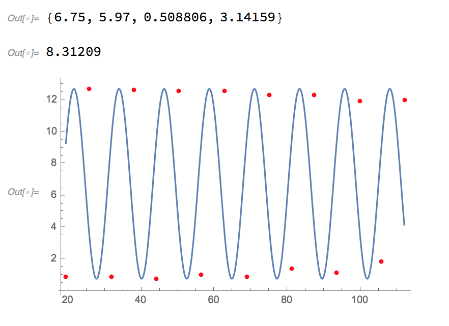
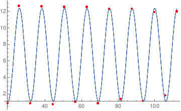
This solution produces reasonable parameters, with the exception of the phase ([CurlyPhi]). Here is a plot of the original data (red dots) with the overlaid Sine curve (blue line). Included also are the values of the four fitted parameters and the root-mean square error.
{displacement, amplitude, \[Omega], \[CurlyPhi]} =
 SinusoidFitDFT[samples]
fittedFunction = (displacement +
     amplitude*Sin[\[Omega]*# - \[CurlyPhi]] &);
RootMeanSquare[yd - fittedFunction /@ xd]
Show[
 ListPlot[samples, PlotStyle -> Red],
 Plot[fittedFunction[x], {x, samples[[1, 1]], samples[[Length@xd, 1]]}]
 ]
It is my understanding that the phase angle of the curve can be obtained by taking the ArcTangent of the result of the Fourier transform at the position of the maximum frequency contributor. Here are the intermediate results. First, the list of frequencies used to construct the transform:
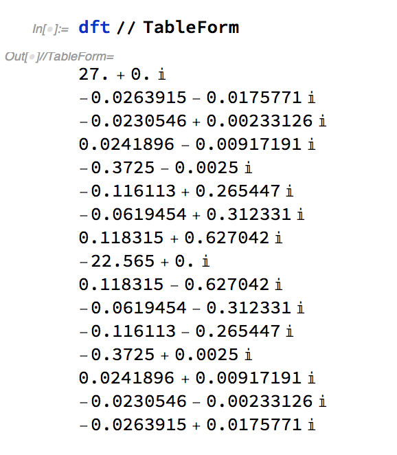
Here is the Fourier transform of the tidal data:
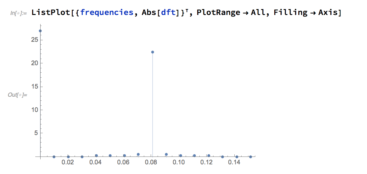
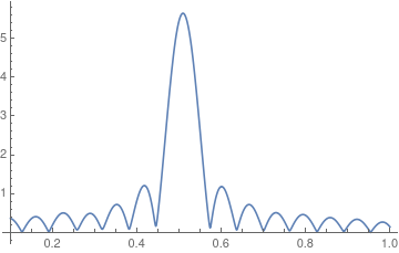
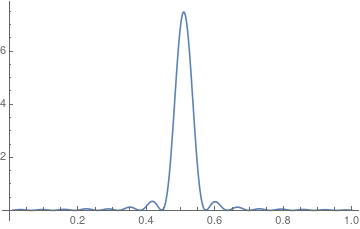
Now the frequency spectrum plot:
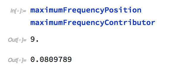
Everything looks okay to this stage. Note that the biggest frequency contributor (besides the zero-frequency component) occurs at the ninth position in the transform. The value of the frequency at this position is at about .08, which naturally corresponds to one high tide about every twelve hours.
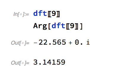
It is my understanding that the phase information for the curve can be obtained by looking at the (two-argument) arctangent of the value of the Fourier transform at this position (available via the Arg function). In the case of the maximum frequency, the phase is [Pi].
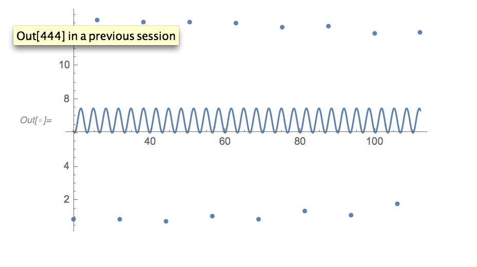
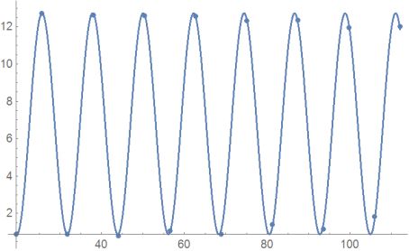
When I look at the original graph, however, it appears that the phase should be -[Pi]/2. That is, the first data point is at near the curve's minimum value. When that value is added into the fitted function, the error is reduced by a factor of twenty.
My questions are: What have I misunderstood about the way that Fourier works? How should I use the Fourier function to fit the data to a sine curve?
BTW, I am aware of this, this and this previous SE questions.
Edit 1:
I ran across an interesting mystery when I tried to refactor the solution provide below by Ulrich Neumann. First, I wrapped his code into the following function call:
MyFunc[] :=
  Module[{J, a, b, om, c, opt},
    J = Sum[(a + b Sin[om xy[[1]] + c] - xy[[2]])^2, {xy, samples}];
    opt = NMinimize[J, {a, b, c, om}];
    {a, b, c, om} /. opt[[2]]
  ];

Show[
  {displacement, amplitude, \[CurlyPhi], \[Omega]} = MyFunc[];
  Plot[
    displacement + amplitude Sin[\[Omega] t + \[CurlyPhi]],
    {t, Min[xd], Max[xd]},
    PlotRange -> All
  ],
  ListPlot[samples]
]
After doing so, the produced plot is identical to that shown in his answer. The anomaly comes when I try to do a simple renaming of a local variable in MyFunc:
MyFunc[] :=
  Module[{J, a, b, cx, c, opt},
    J = Sum[(a + b Sin[cx xy[[1]] + c] - xy[[2]])^2, {xy, samples}];
    opt = NMinimize[J, {a, b, c, cx}];
    {a, b, c, cx} /. opt[[2]]
  ];
Note that the variable om has become cx. When the code is now run, the results look much different:
This strongly violates my intuition that changing a local variable name should not affect the computed results. BTW, I did a Remove["*"];` before each execution to ensure a clean environment. Can anyone explain to me what is happening here?
Edit 2:
I tried a somewhat different approach to get around the problems mentioned by the respondants (unequal increments, incomplete cycles, and too few data points). I took the original data and constructed an interpolation function. I found the roots of this function and extracted values at equally spaced intervals, starting at the first root and continuing through a full number of cycles. I then supplied the extracted values to the Fourier function. Unfortunately the results were no better: the phase angle is still off. The bottom line is that I still don't know how to get a meaningful phase angle out of the Fourier function.


19.4000(the first entry ofxd) which should dictate the phase of the signal, but for your phase analysis you just do a discreteFouriertransform of yourydvalues, which means from the perspective ofFourierthe entries switch from minimum value to maximum value on the grid at Nyquist frequency, which results in the phase angle ofPi. You need to incorporate yourxdvalues to get a meaningful result. $\endgroup$