So In my quest to try to learn some control theory inspired by the following link, I have been modeling an inverse pendulum regulated with a flywheel.
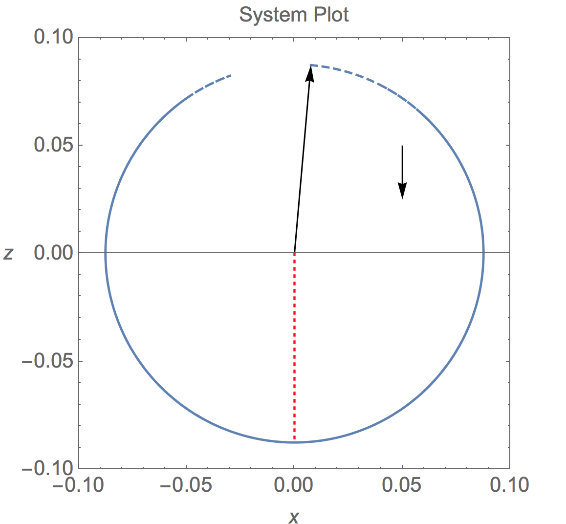
The system model is pretty ok I think, and when doing a parametric plot, shows a result thats close to actual mechanical model I've built.
The red Line is from where my system starts out at, and 85Pi/180 rads is the initial condition for the plot, the black arrow being gravity, and the vector being the centre of gravity of the body.
At this point from here I built my StateSpaceModel to be balanced around the unstable equilibrium Pi and "model" being it's output.
StateSpaceModel[deqns, {{\[Theta][t], \[Pi]}, {\[Theta]'[t],0}, {\[Omega][t],0}, {\[Omega]'[t], 0}}, {u[t], f[t]}, {\[Theta][t]}, t] /. rparams /. params

model = StateSpaceModel[{{{0, 1, 0, 0}, {92.3053, -0.00264558, 0, 2.35457}, {0, 0, 0, 1}, {-92.3053, 0.00264558, 0, -33.6471}}, {{0,0}, {-8.25422,-23.1742}, {0, 0}, {117.954, 23.1742}}, {{1, 0, 0,0}}, {{0, 0}}}, {{\[Theta][t], 0}, Subscript[\[FormalX],1], {\[Omega][t], 0},Subscript[\[FormalX],2]}, {{u[t], 0}, {f[t],0}}, Automatic, t,SamplingPeriod ->None, SystemsModelLabels -> None]
This system has two inputs one, u[t], which is control for the flywheel, and f[t] an outside disturbance.
Here I run into discrepancies,
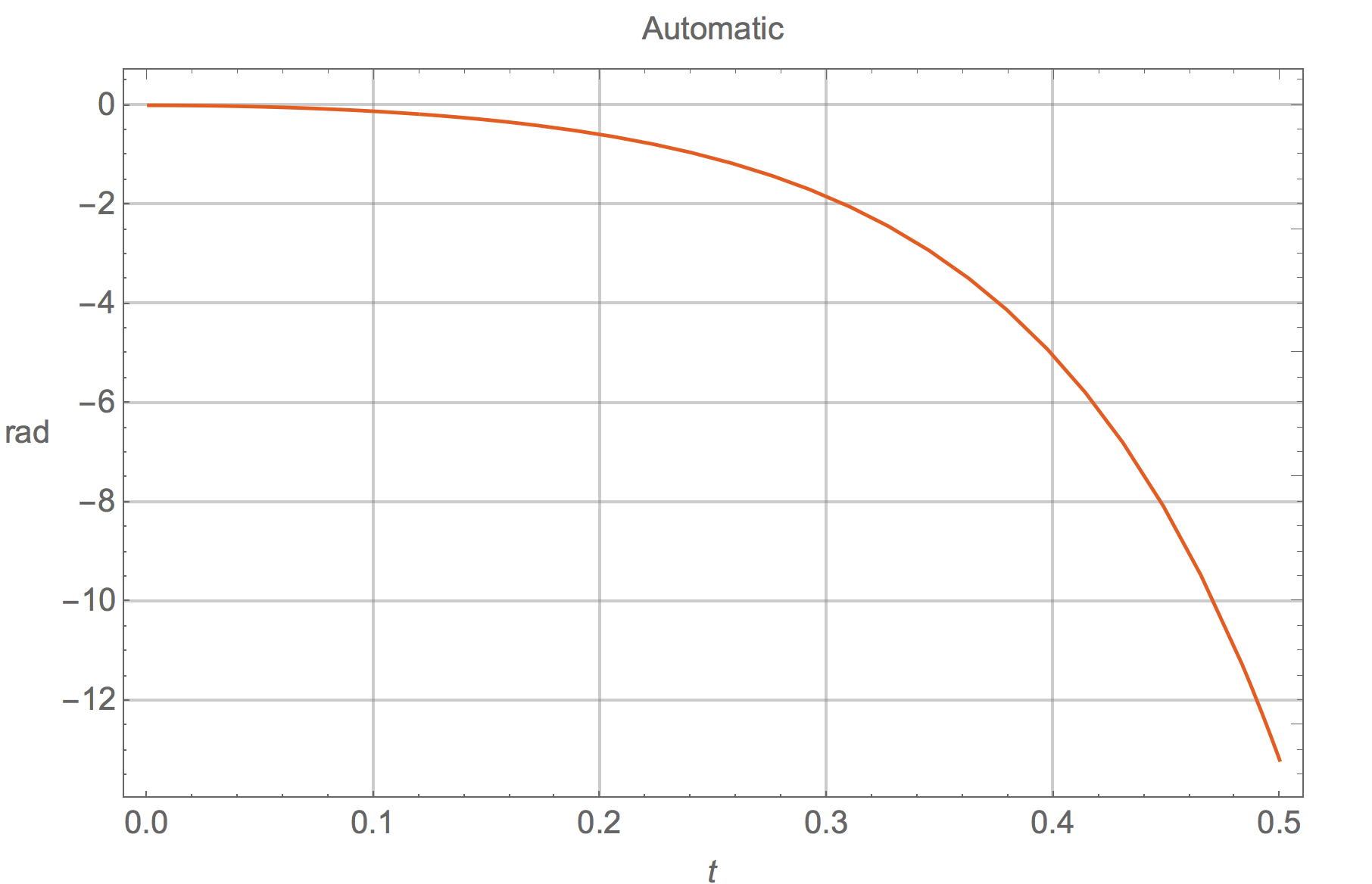
Plot[{OutputResponse[model, {0, 1} UnitStep[t], {t, 0, 6}]}, {t, 0, 0.5}, Evaluated -> True, PlotRange -> All, PlotTheme -> "Scientific",GridLines -> Automatic, ImageSize -> Large, PlotPoints -> 30, RotateLabel -> False, Frame -> True, FrameLabel -> {t, rad,"Automatic"}, LabelStyle -> ( FontSize -> 14)]
This is the result from my system, a UnitStep[t] applied to f[t]. If I allow this to plot more than about a second, I get a result that starts at 0 (though, as I understand it, this Plots deviations around my initial condition) and shoots to 1x10e28 or so. Which of course doesn't make sense since this should just oscillate.
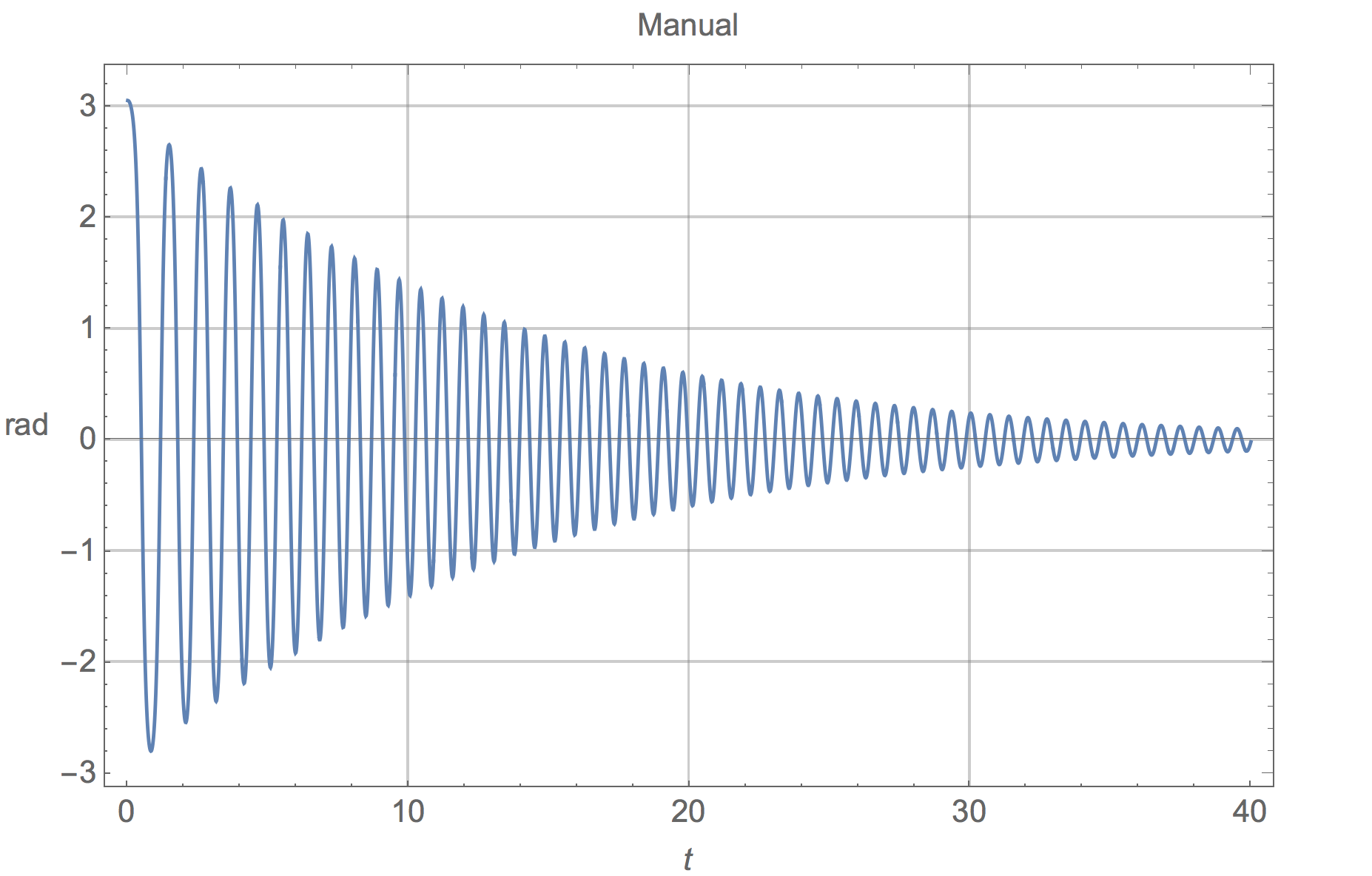
When I plot this 'by hand' I get a result I expect, one that starts at Pi and swings dampened back to zero.
Plot[\[Theta][t] - \[Pi] /. sol, {t, 0, 40}, FrameLabel -> {t, rad,Manual}, GridLines -> Automatic, RotateLabel -> False, ImageSize -> Large, Frame -> True, LabelStyle -> ( FontSize -> 14)]
At this point, I assumed, I've either built the ssm incorrectly, or I'm using OutputResponse incorrectly.
To carry on, I continue to to make the control force via LQR
q = DiagonalMatrix[{1, 100, 100, 0}];
r = {{1}};
gains = Join[LQRegulatorGains[{model, 1}, {q, r}], {ConstantArray[0, 4]}]
controlmodel = SystemsModelStateFeedbackConnect[model, gains];
giving me the gains {{-500.082, -54.8021, -10., -3.12286}, {0, 0, 0, 0}} And the resulting plots with an disturbance force of bumpy[t]
bumpy[t_] := 2 E^(-10 (t - 3)^2) - 1 E^(-10 (t - 6)^2) + 2 E^(-10 (t-9)^2)
Orange is theta, the pendulum body, and omega the flywheel rad/s
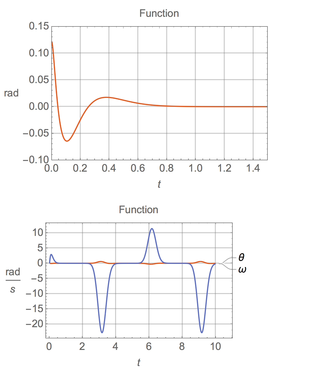
This seems like an excellent control and a excellent proof of control concept (for me anyways). Manually plotting with this $controlforce$.
controlforce = -gains[[1]].{\[Theta][t] - \[Pi], \[Theta]'[t], \[Omega][t], \[Omega]'[t]}


500.082 (-\[Pi] + \[Theta][t]) + 10. \[Omega][t] + 54.8021 Derivative[1][\[Theta]][t] + 3.12286 Derivative[1][\[Omega]][t]
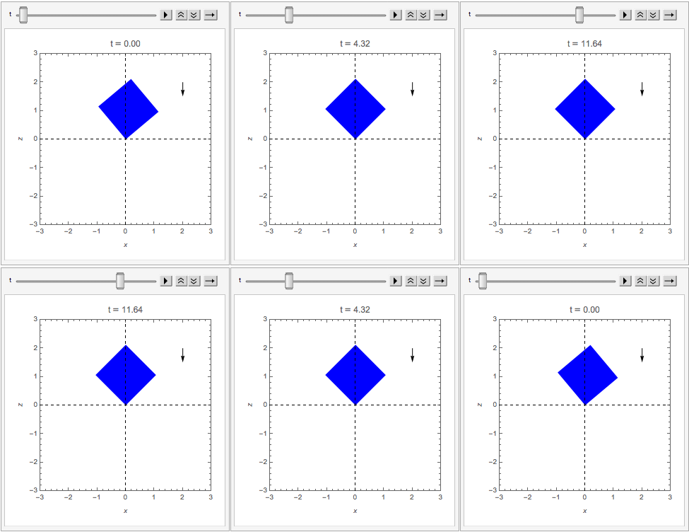
Simulating/animating this gives me (forgive the poor frame rate) also, again something I expected:
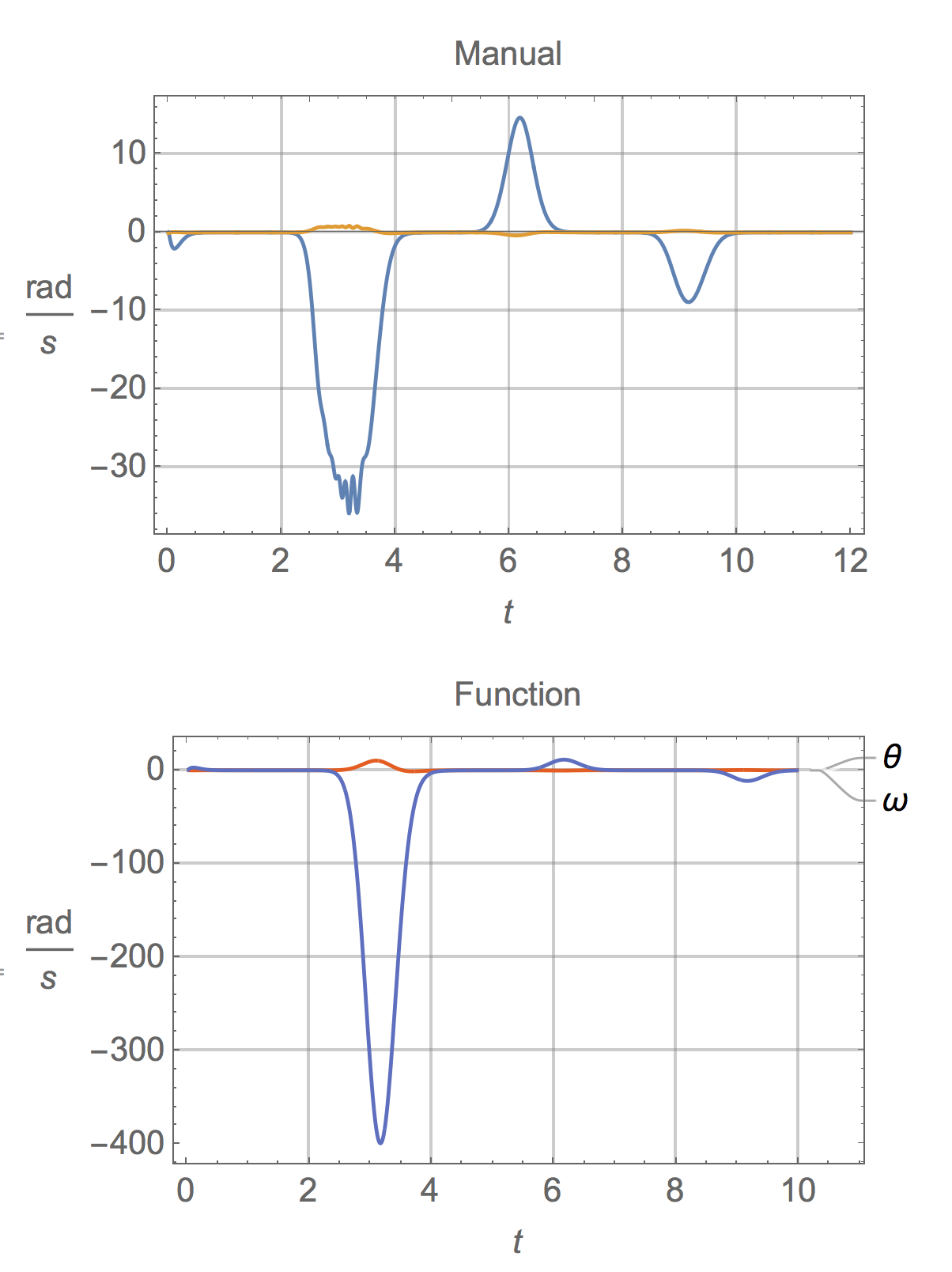
Now to find out where this system fails I increase bumpy[t bumpy[t_] := 35 E^(-10 (t - 3)^2) - 1 E^(-10 (t - 6)^2) + 1 E^(-10 (t - 9)^2)
Like the initial difference between my manual plot, and the OutputResponse of the system without control.
I now have in the StateResponse of omega going to about 400rad/s and my manual plot with the control forces going to 30rad/s and a weird stuttering but recovering.
(400 rad/s is about half of what the motors can achieve, though, the system highly unlikely wouldn't recover from this kind of force, but thats why I'm trying to find out at what point this system fails)
So long story short and to the question, Whats going wrong in my modeling/simulation?
OutputResponse isn't giving me a correct oscillating response. StateResponse and my manual plot sync well up until a certain disturbance force, where I expect both to spectacularly fail, at this point, I don't know which model I can trust.
If you'd like to see all of my code and the initial model with Lagrangian built PDE, I can gladly post a link of the file if the initial SSM isn't sufficient.
I greatly appreciate the help!

