I am trying to plot data using the ListLogLinearPlot.
Here is my initial code:
 ListLogLinearPlot[{xlist, ynorm}\[Transpose],
   PlotRange -> All,
   Joined -> True,
   Axes -> {0, 0},
   PlotStyle -> {{Thick, Black}, {Black}}, Frame -> True,
   FrameLabel -> {"Size (d,nm)", "Normalized Signal Intensity"},
   LabelStyle -> Directive[Bold, 20, FontFamily -> "Arial", Black]]
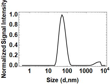
and my result is:
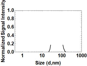
Now, when I try to change the range to go from 0 to 1000 on the x-axis, the plot becomes this:
ListLogLinearPlot[{xlist, ynorm}\[Transpose],
  PlotRange -> {{0, 1000}, {0.0, 1.0}},
  Joined -> True,
  Axes -> {0, 0},
  PlotStyle -> {{Thick, Black}, {Black}}, Frame -> True,
  FrameLabel -> {"Size (d,nm)", "Normalized Signal Intensity"},
  LabelStyle -> Directive[Bold, 20, FontFamily -> "Arial", Black]]
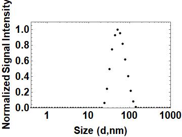
If I remove Joined-> True, I get the requested plot range, but I want my plot to be joined.
ListLogLinearPlot[{xlist, ynorm}\[Transpose],
  PlotRange -> {{0, 1000}, {0, 1.1}},
  Axes -> {0, 0},
  PlotStyle -> {{Thick, Black}, {Black}}, Frame -> True,
  FrameLabel -> {"Size (d,nm)", "Normalized Signal Intensity"},
  LabelStyle -> Directive[Bold, 20, FontFamily -> "Arial", Black]]
I have no idea of what is going on. I am a polymer chemist by trade and know very basic coding. All I want is to be able to import light scattering data and visualize it using Mathematica.
Edit: Thank you for all your help! I apologize for not including my x and y data lists; here they are:
xs
{0.4, 0.463, 0.536, 0.621, 0.719, 0.833, 0.965, 1.117, 1.294, 1.499, \
1.736, 2.01, 2.328, 2.696, 3.122, 3.615, 4.187, 4.849, 5.615, 6.503, \
7.531, 8.721, 10.1, 11.696, 13.545, 15.686, 18.166, 21.037, 24.363, \
28.214, 32.674, 37.84, 43.821, 50.748, 58.771, 68.061, 78.82, 91.28, \
105.709, 122.42, 141.772, 164.183, 190.137, 220.194, 255.002, \
295.312, 341.995, 396.058, 458.666, 531.172, 615.139, 712.379, \
824.992, 955.406, 1106.44, 1281.34, 1483.89, 1718.47, 1990.12, \
2304.72, 2669.04, 3090.96, 3579.58, 4145.44, 4800.75, 5559.64, \
6438.51, 7456.3, 8634.99, 10000.}
ys
{0., 0., 0., 0., 0., 0., 0., 0., 0., 0., 0., 0., 0., 0., 0., 0., 0., \
0., 0., 0., 0., 0., 0., 0., 0., 0., 0., 0., 0.947, 3.55, 7.16, \
10.711, 13.27, 14.293, 13.678, 11.701, 8.885, 5.849, 3.167, 1.248, \
0.246, 0., 0., 0., 0., 0., 0., 0., 0., 0., 0., 0., 0., 0., 0., 0., \
0., 0.04, 0.136, 0.282, 0.461, 0.649, 0.817, 0.941, 0.998, 0.971, 0., \
0., 0., 0.}


{xlist,ynorm}might be plausible in side, is there any chance you might edit your question to include that data? Then someone could use their MMA to try to reproduce exactly your problem and see if the could find a fix that would be far more likely to work. $\endgroup$Joined-.Trueand post-process the output to turnPoints into aLine, e.g.,ListLogLinearPlot[{xlist, ynorm}\[Transpose], PlotRange -> {{0, 1000}, {0.0, 1.0}}, Axes -> {0, 0}, PlotStyle -> {{Thick, Black}, {Black}}, Frame -> True, FrameLabel -> {"Size (d,nm)", "Normalized Signal Intensity"}, LabelStyle -> Directive[Bold, 20, FontFamily -> "Arial", Black]] /. Point -> Line$\endgroup$PlotRange -> {{0, 1000}, {0.0, 1.0}}thexminis0; there is no0on a log plot. If you change this to a positive value, does the problem go away? Or tryPlotRange -> {Automatic, {0.0, 1.0}}$\endgroup$