Fitting data to an ARProcess using FindProcessParameters

Question

I have 50 data points that I would like to represent as an AR(4) process. I'd like to over-plot the behaivor of the estimated process model with that of the original (raw) data before I use the model to predict 10 days into the future.

Remove[a1, a2, a3, a4, v]
processdata = {{1, 5.0}, {2, 9.0}, {3, 8.0}, {4, 10.0}, {5, 6.1}, {6, 
10.4}, {7, 9.1}, {8, 11.6}, {9, 7.5}, {10, 12.1}, {11, 10.4}, {12,
 13.5}, {13, 9.0}, {14, 14.1}, {15, 11.9}, {16, 15.7}, {17, 
10.8}, {18, 16.4}, {19, 13.7}, {20, 18.3}, {21, 12.9}, {22, 
19.0}, {23, 15.8}, {24, 21.2}, {25, 15.3}, {26, 22.1}, {27, 
18.3}, {28, 24.6}, {29, 18.1}, {30, 25.8}, {31, 21.2}, {32, 
28.6}, {33, 21.4}, {34, 30.0}, {35, 24.6}, {36, 33.2}, {37, 
25.2}, {38, 35.0}, {39, 28.6}, {40, 38.5}, {41, 29.6}, {42, 
40.7}, {43, 33.3}, {44, 44.7}, {45, 34.8}, {46, 47.4}, {47, 
38.8}, {48, 52.0}, {49, 40.9}, {50, 55.2}};
plot1 = ListPlot[processdata, Joined -> True, Frame -> True, 
FrameLabel -> {"Time (days)", "Temperature"}, AxesOrigin -> {0, 0}, 
PlotRange -> All, PlotStyle -> {Thick, Red}, 
PlotLabel -> "Plot 1: Raw Process Data"]

Here I use FindProcessParameters to estimate the four coefficients and the variance. Then I use these values to see how well the model matches the raw data.

params = FindProcessParameters[processdata, 
ARProcess[{a1, a2, a3, a4}, v]]
a1 = params[[1, 2]];
a2 = params[[2, 2]];
a3 = params[[3, 2]];
a4 = params[[4, 2]];
v = params[[5, 2]];
sigma = Sqrt[v];
y = Table[0, {50}];
y[[1]] = 5.0;
y[[2]] = 9.0;
y[[3]] = 8.0;
y[[4]] = 10.0;
dist = NormalDistribution[0, sigma];
t = 4;
Do[{
t = t + 1,
If[t > 50, Break[]],
whitenoise = RandomVariate[dist],
y[[t]] = whitenoise/(
1 - (a1*y[[t - 1]]) - (a2*y[[t - 2]]) - (a3*y[[t - 3]]) - (a4*
   y[[t - 4]]))},
{100}];
modeldata = Transpose[{Range[Length[y]], y}];
plot2 = ListPlot[modeldata, Joined -> True, Frame -> True, 
FrameLabel -> {"Time (days)", "Temperature"}, 
AxesOrigin -> {0, -40}, PlotRange -> All, 
PlotStyle -> {Thin, Black}, PlotLabel -> "Plot 2: Model Data"];
plot3 = Show[plot1, plot2, 
PlotLabel -> "Plot 3: Raw Process Data(Red) vs AR Model(Black)", 
AxesOrigin -> {0, -80}]

The above model performance is not very good. Am I doing something wrong here ? I then tried specifying MaximumLikelihood as the process estimator in the hope of getting better parameter estimates but get a FindArgMax error message which I also don't understand.

Remove[a1, a2, a3, a4, v]
params = FindProcessParameters[processdata, 
ARProcess[{a1, a2, a3, a4}, v], 
ProcessEstimator -> "MaximumLikelihood"]

FindArgMax::nrnum: "The function value {-Log[PDF[ARProcess[{0.746727,0.814726, . . .

I'm not a Mathematica power user or time-series expert so relatively gentle answers would be much appreciated. Thanks.

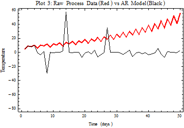
Edit 1: Now that I have more than 10 reputation points (I'm a first time stackexchange user) I'm now able to show a plot of the AR model performance.

Since the AR model has a probabilistic component (the white noise), a plot that you may generate will in all likelihood look different than above, nonethless I would expect the fit to still be poor. The question is why ?

Answer 1

There are a couple issues here worth touching on, I think.

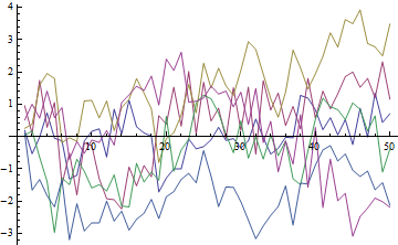
Firstly, you are making things overly complicated for your self. Mathematica has a built in function for generating data from a random process, called RandomFunction. You can easily use it and a time series model to generate data, like so:

armodel = 
  ARProcess[{0.5469865826154379`, 
    0.5394047756716838`, -0.41857450624035714`, 0.2598799117296679`}, 
   0.5235408772937131`];
samples = RandomFunction[armodel, {1, 50}, 6];
ListLinePlot[samples]

This also helps show the first part of the answer to why your model doesn't fit the data. The $AR(4)$ model is very general and fits a infinite number of different time series. All time series models are essentially linear combinations of normal random numbers. There is no reason to assume a linear combination of one set of random numbers would look much like the same linear combination of a different set of random numbers.

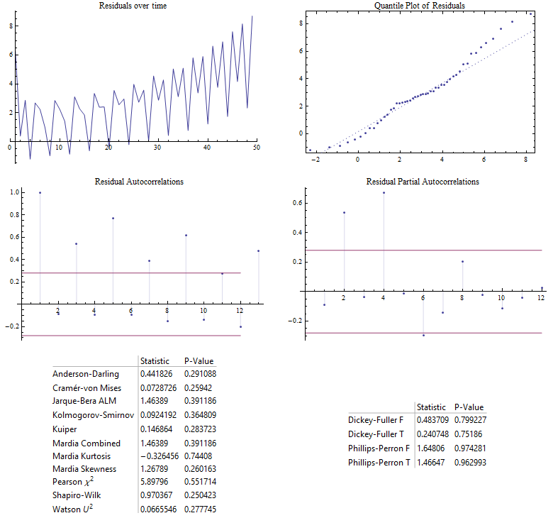
The correct way to test the fit of a time series model is to look at the residuals of your data when you filter with the model. The residuals should look like independent normal random numbers. I wrote a function which combine some of the diagnostic tools available in Mathematica to help test the fits of a model to the data:

residualAnalysis[model_, data_List] := Module[
  {res, len, lag, interval},
  res = Rest[data - KalmanFilter[model, data]];
  len = Length@res;
  lag = Floor[len/4];
  interval = 1.96/Sqrt[len];
  GraphicsGrid[
   {
    {
     ListLinePlot[res, PlotRange -> All, ImageSize -> Medium, 
      PlotLabel -> "Residuals over time"],
     QuantilePlot[res, ImageSize -> Medium, 
      PlotLabel -> "Quantile Plot of Residuals"]
     },
    {
     Show[
      ListPlot[CorrelationFunction[res, {lag}], Filling -> 0, 
       PlotRange -> All, AxesOrigin -> {0, 0}, 
       PlotLabel -> "Residual Autocorrelations", ImageSize -> Medium],
      Plot[{-interval, interval}, {x, 0, lag}, 
       PlotStyle -> {ColorData[1, 2], ColorData[1, 2]}]
      ],
     Show[
      ListPlot[PartialCorrelationFunction[res, {lag}], Filling -> 0, 
       PlotRange -> All, AxesOrigin -> {0, 0}, 
       PlotLabel -> "Residual Partial Autocorrelations", 
       ImageSize -> Medium],
      Plot[{-interval, interval}, {x, 0, lag}, 
       PlotStyle -> {ColorData[1, 2], ColorData[1, 2]}]
      ]
     },
    {
     DistributionFitTest[res, Automatic, {"TestDataTable", All}],
     UnitRootTest[data, Automatic, {"TestDataTable", All}]
     }
    }
   ]
  ]

You can use it like so:

data = {{1, 5.0}, {2, 9.0}, {3, 8.0}, {4, 10.0}, {5, 6.1}, {6, 
     10.4}, {7, 9.1}, {8, 11.6}, {9, 7.5}, {10, 12.1}, {11, 
     10.4}, {12, 13.5}, {13, 9.0}, {14, 14.1}, {15, 11.9}, {16, 
     15.7}, {17, 10.8}, {18, 16.4}, {19, 13.7}, {20, 18.3}, {21, 
     12.9}, {22, 19.0}, {23, 15.8}, {24, 21.2}, {25, 15.3}, {26, 
     22.1}, {27, 18.3}, {28, 24.6}, {29, 18.1}, {30, 25.8}, {31, 
     21.2}, {32, 28.6}, {33, 21.4}, {34, 30.0}, {35, 24.6}, {36, 
     33.2}, {37, 25.2}, {38, 35.0}, {39, 28.6}, {40, 38.5}, {41, 
     29.6}, {42, 40.7}, {43, 33.3}, {44, 44.7}, {45, 34.8}, {46, 
     47.4}, {47, 38.8}, {48, 52.0}, {49, 40.9}, {50, 55.2}}[[All, 2]];
model = EstimatedProcess[data2, ARProcess[{a1, a2, a3, a4}, v]];
residualAnalysis[model, data]

This also answer the second part of why your question of why the model doesn't fit your data. The model is inappropriate for the data. A $AR(4)$ is stationary, meaning the mean and variance do not change over time, which is not the case with your data. In your data both mean and variance is increasing. Some amount of differencing and transformation of the data would be needed to deal with that. You can also see from the Residuals over time plot and the Residual Autocorrelation plot that there seems to be a very strong seasonal part in the data that ought to be included in the model. The Partial Autocorrelation plot also shows several remaining significant spikes.

Honestly, looking at your data it doesn't look random at all. It looks wholly deterministic. You would get far better predictions fitting a deterministic model to the data and use that for predictions.

Answer 2

I think your modeldata generation should be

y[[t]] = whitenoise + (a1*y[[t-1]]) + (a2*y[[t-2]]) + (a3*y[[t-3]]) + (a4*y[[t-4]])

since for an AR(4) model, the current value is a linear combination of four previous values plus the current value of the noise.

Also, after looking at the plot of processdata, I observed strong trend and seasonality, so you may want to consider differencing the data before fitting AR(4) or other stationary time series.