So I am a beginner with stochastic differential equations and came across Mathematica's capabilities for solving them. I am solving the stochastic Mathieu equation with a harmonic forcing term that has a stochastic fluctuation imposed.
The linear set of ODEs to solve this are (ready for Ito form):
$ dx(t)=y(t) dt,\\ dy(t)=\lambda (t) dt \cos (\nu t) \sin (x(t))-\epsilon \,\textbf{dw(t)} \sin (x(t))$
Where $\lambda$ is time-varying as in the code below. $\nu$ possesses some physical characteristic I cannot place at the moment but takes real values. $\epsilon$ is a small number $<<1$. $w$ is the Wiener process distribution with zero drift and volatility (Ariaratnam et al.) (google drive link to paper. Only introduction is relevant for now.).
tmax = 100;
\[Lambda][t_] :=
 Piecewise[{{.95, t <= tmax/4}, {1.1, tmax/4 < t <= tmax/2}, {1.25,
    t > tmax/
      2}}]; \[Nu] = 105.; \[Epsilon] = 0.001; x0 = 0.1; y0 = 0.1; \
drift = 0; volatility = 1.;

sme = ItoProcess[
   {
    \[DifferentialD]x[t] == y[t] \[DifferentialD]t,
    \[DifferentialD]y[
       t] == \[Lambda][t] Cos[\[Nu] t] Sin[
        x[t]] \[DifferentialD]t - \[Epsilon] Sin[
        x[t]] \[DifferentialD]w[t]
    }, x[t],
   {{x, y}, {x0, y0}},
   {t, 0}, w \[Distributed] WienerProcess[drift, volatility]
   ];
path = RandomFunction[sme, {0., tmax, 1}, 1]
My main issue is with the path = RandomFunction[sme, {0., tmax, 1}, 1] line. Here, it is my understanding that the {0., tmax, 1} is a time-stepping from 0 to tmax in steps of 1.
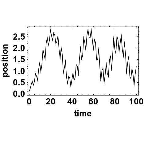
With a "time-step" of 1, I get the following dynamics which are reasonable, I would think:
ListLinePlot[path, PlotRange -> All, GridLines -> None,
 ImageSize -> 250 {1, 1}, Frame -> True, FrameStyle -> Black,
 FrameLabel -> {"time", "position"},
 PlotStyle -> {Thickness[0.005], Black},
 BaseStyle -> {FontSize -> 14, Bold}, Axes -> False]
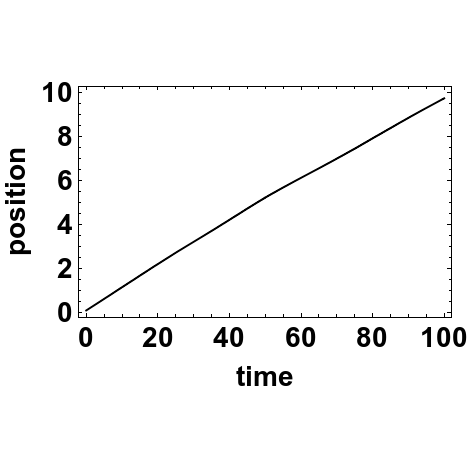
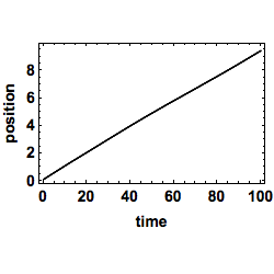
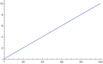
However, if I change the time-step to, say, 0.1, I see an instability (or is it?) with some sort of monotonically increasing position.
Am I going wrong somewhere? Any input or assistance, I am grateful for.
Edit: The position plot is for x[t].

