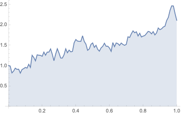
This shows how it works:
proc = ItoProcess[\[DifferentialD]X[
     t] == -α WhenEvent[x[t] == 1.,
      x[t] -> -x[t]] Exp[-α t] Log[X0/K] X[
      t] \[DifferentialD]t + σ X[t] \[DifferentialD]W[t],
  X[t], {X, X0}, t, W \[Distributed] WienerProcess[]]
Mean[proc[t]]
PDF[proc[t], x]
proc1 = proc /. {X0 -> 70, K -> 2, σ -> 0.1, α -> 0.3};
DiscretePlot[PDF[proc1[t], x], {x, 0, 10}]
CovarianceFunction[proc1, s, t]
The DiscretePlot is very time-consuming, so I shortened that. Definitely this does not work if the questions target to use RandomFunction.
Plot3D[CovarianceFunction[proc1, s, t], {s, 0, 5}, {t, 0, 5}, ColorFunction -> "Rainbow"]
The equation given in the question might not work because the denominator is singular at infinitely many points. Mathematica works on the Complexes.
In this methodolgoy Mod is an alternative.
proc4 = ItoProcess[\[DifferentialD]x[t] ==
   Sin[Mod[x[t], \[Pi]]]/(
     1 - Cos[Mod[x[t], \[Pi]]]) \[DifferentialD]t + \[DifferentialD]w[
      t], x[t], {x, 1}, t, w \[Distributed] WienerProcess[]]
(* ItoProcess[{{-(
Sin[Mod[x[t], [Pi]]]/(-1 + Cos[Mod[x[t], [Pi]]]))}, {{1}},
x[t]}, {{x}, {1}}, {t, 0}] *)
RandomFunction[proc4, {0., 1., 0.01}]

Further extended:
    f[x_] := Piecewise[Table[{Sin[x - n*Pi - \[Epsilon]]/(1 - Cos[x - n*Pi - \[Epsilon]]),
     -Pi + n*Pi + \[Epsilon] <= x <= Pi + n*Pi + \[Epsilon]}, {n, -5, 5}]]
Plot[f[x], {x, -6*Pi + \[Epsilon], 6*Pi + \[Epsilon]}]
works too with the RandomProcess representation and therefore complete. But still the problem remains that the function is singular for 2 n 𝜋, Element[n,Integers].
ListLinePlot[%, Filling -> Axis]

Using the Fourier make this ideally periodic. For example:
p = Table[
   f[x], {x, \[Epsilon],
    6 \[Pi] + \[Epsilon], (6 \[Pi] + \[Epsilon])/999}];
s = Fourier[p];
ListPlot[Abs[InverseFourier@s], PlotRange -> Full]
And the use this as an InterpolatingFunction of x: Interpolation@InverseFourier@s.


RandomFunctionon SDE does not seem to be programmed to handle events. (In the example you might be able to post-process the time series, but that seems rather specific to the SDE and event.) $\endgroup$