5
$\begingroup$

I have a large $2^N \times 2^N$ matrix. It is the exact Hamiltonian of a spin chain model which I have generated with code I wrote in Fortran. The code block diagonalizes the Hamiltonian into constant total-spin sectors and furthermore into blocks of definite momentum. I wish to diagonalize it (find the eigenvalues), however when I import it into Mathematica and apply Eigenvalues[] to it, it takes a very long time. I assume that it would be much much faster to just compute the eigenvalues of each block individually (currently modifying my Fortran code to separate these blocks). For example, for $N=10$ the matrix is $1028\times 1028$, but the largest block is $25\times 25$ and there are (I think) N(N+1) = 110 blocks, most of which are maybe $5\times 5$. Is there a way to indicate to Mathematica that the matrix is block diagonal, or an efficient way to do this without actually putting each block in a separate file and importing and diagonalizing all of them separately?

Note that the matrix is Hermitian and may be complex.

$\endgroup$
2
  • 1
    $\begingroup$ "when I import it into Mathematica" - is it a SparseArray[] when you import it? $\endgroup$ Commented Mar 28, 2018 at 19:23
  • $\begingroup$ I imported it as a table, I tried converting it to a SparseArray[] before passing it to Eigenvalues[] but I got a message which said that it was being converted back into a normal matrix because it would be faster. I am currently modifying my code so that it can be stored as a sparse array since only around ~1% of the matrix elements are non-zero. $\endgroup$
    – Kai
    Commented Mar 28, 2018 at 19:58

1 Answer 1

5
$\begingroup$

Here is one possible approach. First, a random matrix that can be sorted into a block diagonal matrix (so that you don't have to worry about converting it to block diagonal form when importing):

sa = With[{perm=PermutationList[RandomPermutation[50],50]},
    SparseArray @ ArrayFlatten[
        DiagonalMatrix[Table[a,10]] /. a :> RandomReal[1,{5,5}]
    ][[perm,perm]]
];

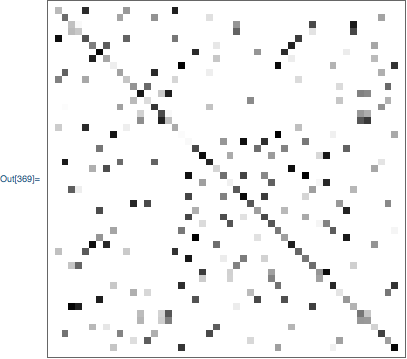
Here is a view of the nonzero elements:

ArrayPlot[sa]

enter image description here

Now, we can use AdjacencyGraph to convert to a graph, and then ConnectComponents to find the blocks:

blocks = ConnectedComponents @ AdjacencyGraph @ Unitize @ sa

{{22, 26, 32, 39, 40}, {20, 25, 28, 31, 37}, {13, 16, 17, 45, 46}, {12, 14, 29, 42, 49}, {9, 19, 33, 41, 50}, {7, 21, 30, 34, 43}, {6, 8, 24, 35, 47}, {3, 4, 27, 38, 44}, {2, 10, 15, 23, 48}, {1, 5, 11, 18, 36}}

Finally, we can use these blocks to find the eigenvalues:

eigs = Eigenvalues[sa[[#, #]]]& /@ blocks

{{1.99765 + 0. I, 0.658726 + 0. I, -0.412903 + 0.13731 I, -0.412903 - 0.13731 I, 0.253 + 0. I}, {2.84384 + 0. I, -0.75531 + 0. I, 0.261846 + 0.53826 I, 0.261846 - 0.53826 I, 0.170376 + 0. I}, {2.23096, 0.481537, 0.240699, -0.220823, 0.0584065}, {1.79549 + 0. I, -0.32683 + 0. I, 0.113261 + 0.30506 I, 0.113261 - 0.30506 I, -0.0047193 + 0. I}, {2.52376 + 0. I, -0.80018 + 0. I, 0.492073 + 0.32248 I, 0.492073 - 0.32248 I, -0.300104 + 0. I}, {2.95724 + 0. I, -0.534463 + 0. I, 0.215221 + 0.394219 I, 0.215221 - 0.394219 I, -0.0152984 + 0. I}, {2.46332 + 0. I, -0.594371 + 0. I, 0.0462041 + 0.1835 I, 0.0462041 - 0.1835 I, 0.106778 + 0. I}, {2.26045 + 0. I, -0.917553 + 0. I, 0.100373 + 0.481719 I, 0.100373 - 0.481719 I, 0.423527 + 0. I}, {2.25639 + 0. I, 0.34116 + 0.468159 I, 0.34116 - 0.468159 I, 0.458043 + 0. I, -0.0805449 + 0. I}, {2.4259 + 0. I, -0.334963 + 0.331565 I, -0.334963 - 0.331565 I, 0.462109 + 0. I, -0.109226 + 0. I}}

Let's compare with using Eigenvalues directly on the matrix:

Block[{Internal`$EqualTolerance=4},
    Sort@Eigenvalues[sa] == Sort@Flatten@eigs
]

True

$\endgroup$
9
  • $\begingroup$ Internal`$EqualTolerance is cool. Never knew about that one. $\endgroup$
    – b3m2a1
    Commented Mar 28, 2018 at 23:53
  • 1
    $\begingroup$ @b3m2a1 I think so too. It allows one to use the more instructive equal comparison instead of checking that the max of the absolute value of the differences is small. $\endgroup$
    – Carl Woll
    Commented Mar 28, 2018 at 23:55
  • $\begingroup$ @b3m2a1, for reference, there's also Internal`$SameQTolerance. $\endgroup$ Commented Mar 29, 2018 at 0:37
  • $\begingroup$ wow I did not know about pretty much any of these functions haha, I need to take some time to understand how this works and how to apply it to my problem. Thank you. ConnectedComponents is pretty darn cool. $\endgroup$
    – Kai
    Commented Mar 29, 2018 at 1:32
  • $\begingroup$ A shorter, but undocumented way to get the connected components: Union[sa["AdjacencyLists"]] $\endgroup$ Commented Mar 29, 2018 at 3:29

Your Answer

By clicking “Post Your Answer”, you agree to our terms of service and acknowledge you have read our privacy policy.

Not the answer you're looking for? Browse other questions tagged or ask your own question.