3
$\begingroup$

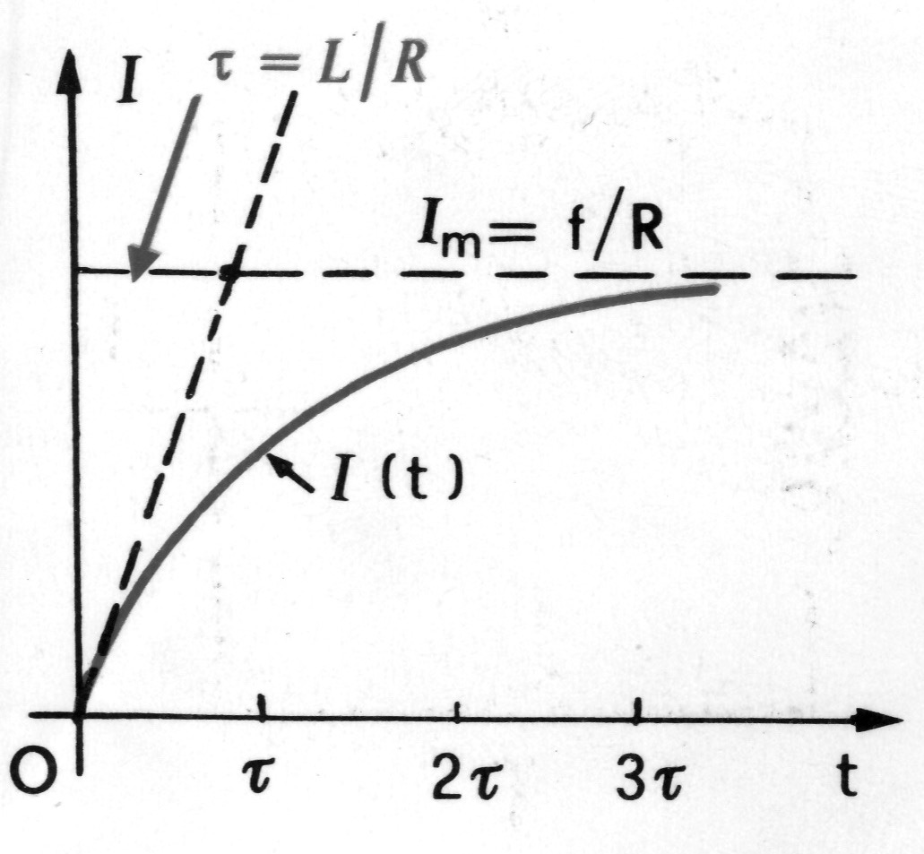
I would like to make a plot such as the one in the picture below:

enter image description here

Note that there no ticks on the y-axis and the x-axis ticks are expressed in term of a parameter -- the function being presented as if it were evaluated only qualitatively and the plot can be considered to be of a function describing a general phenomenon.

I tried with

F[t_] = Imax (1 - Exp[-t/tau])
Plot[F[t], {t, 0, 3 tau}] 

but obviously that was not the correct way to do it. Is it possible to do such a thing with Mathematica?

$\endgroup$
2
  • 1
    $\begingroup$ The last two examples in the Scope > Ticks Positions and Labeling section of the docs, reference.wolfram.com/language/ref/Ticks.html, shows how to do it. $\endgroup$
    – Michael E2
    Commented Jun 7, 2017 at 17:04
  • $\begingroup$ Hi, welcome to Mathematica.SE, please consider taking the tour so you learn the basic rules of the site. Once you gain enough reputation by making good questions you will be able to vote up and down both questions and answers. Your question has been answered, but its a good idea to wait 24hours for other answers before accepting the best one for you. (Notice the links to useful information) $\endgroup$
    – rhermans
    Commented Jun 7, 2017 at 17:53

3 Answers 3

4
$\begingroup$

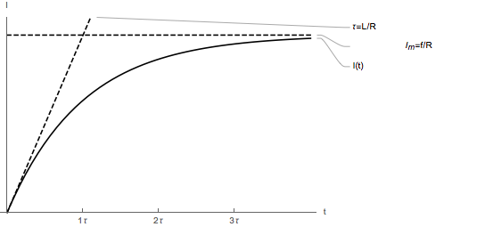
For plots like this you're plotting in units of Imax, and tau so replace t/tau with t'=t/tau then t'=1 when t=tau etc. You can use ticks to indicate this. Imax is just a scaling parameter, so leave it as 1 and everything is relative to Imax:

Plot[
 {Callout[(1 - Exp[-t]), "I(t)"], Callout[t, "τ=L/R"], 
  Callout[1, "Im=f/R"]}
 ,
 {t, 0, 4},
 Ticks -> {
   {#, ToString@# <> "τ"} & /@ Range[3],
   None}
 , AxesLabel -> {"t", "I"}
 , PlotRange -> {0, 1.1}
 , PlotStyle -> {Black, Directive[Black, Dashed], 
   Directive[Black, Dashed]}
 ]

enter image description here

The Callouts are a little wonky in this example, but they are the simplest way to label curves like this.

$\endgroup$
2
  • 1
    $\begingroup$ For those who are picky, the following give the labels & ticks displayed the way they're suppose to display in TraditionalForm: Ticks -> {{#, # * HoldForm[\[Tau]]} & /@ Range[3], None} and AxesLabel -> {Automatic, DisplayForm@RowBox[{"I"}]}. (If you're really picky, use MaTeX.) $\endgroup$
    – Michael E2
    Commented Jun 7, 2017 at 18:45
  • $\begingroup$ Your solution was exactly what I was looking for! $\endgroup$ Commented Jun 12, 2017 at 18:07
7
$\begingroup$

You must use a numerical value for plotting, but you can easily label your axes with whatever you want in this form:

Ticks-> {{{1, "τ"},{2, "2τ"},{3, "3τ"}}, Automatic}

Incidentally, what is the value of Imax?

Plot[{1, x Cos[5 π/16], Exp[-1/x]}, 
{x, 0, 3}, 
PlotStyle -> {Dashed, Automatic, Automatic}, 
Ticks -> {{{1, "τ"}, {2, "2τ"}, {3, "3τ"}}, None}, 
Epilog -> {Text @@@ 
          {{"t = L/R", {0.5, 1.3}}, 
           {"I(t)", {1.4, 0.3}}, 
           {"Im = f/R", {2.5, 1.1}}}, 
           Arrow /@ 
          {{{0.5, 1.3}, {0.2, 1}}, 
          {{1.4, 0.3}, {1.2, 0.4}}}}]
$\endgroup$
3
  • $\begingroup$ Thanks anyway. Are you 100% sure there is no way to get a generic plot, but labelling after the plot is done? By the way, Imax It's just the asymptotic value that the function approaches as t goes to infinity! $\endgroup$ Commented Jun 7, 2017 at 17:24
  • $\begingroup$ It's the trend of the current in a LR circuit with constant voltage $\endgroup$ Commented Jun 7, 2017 at 17:25
  • 1
    $\begingroup$ Absolutely positive there's no way to get a plot with a generic (unspecified) variable. After all, how could the software know where to plot a point? You can, of course, define your variables beforehand (e.g., tau = 1;) and then apply your Plot referring to these values, but generically, absolutely not. Imagine plotting $1/(x - q)$ versus $x$ and not knowing the numerical value of $q$ (whether it was positive or negative or zero)!! $\endgroup$ Commented Jun 7, 2017 at 17:26
1
$\begingroup$

You can create each graphic instance and show them together. Though, as far as I know, you must provide numerical values. Then its a matter of tweaking values to get the graphics you want.

p1 = Plot[1, {x, 0, 3}, PlotStyle -> Dashed, 
  Ticks -> {{{1, "τ"}, {2, "2τ"}, {3, "3τ"}}, 
    Automatic}] (*only one plot needs the ticks*)
p2 = Plot[x*Cos[5 Pi/16], {x, 0, 3}, PlotStyle -> Dashed]
p3 = Plot[1/Exp[1/x], {x, 0, 3}]
t1 = Graphics[Text["t = L/R", {0.5, 1.3}]]
t2 = Graphics[Text["I(t)", {1.4, 0.3}]]
t3 = Graphics[Text["Im = f/R", {2.5, 1.1}]]
a1 = Graphics[Arrow[{{0.5, 1.3}, {0.2, 1}}]]
a2 = Graphics[Arrow[{{1.4, 0.3}, {1.2, 0.4}}]]
Show[p1, p2, p3, t1, t2, t3, a1, a2]

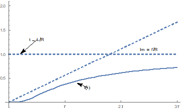
output

$\endgroup$
2
  • 2
    $\begingroup$ Far simpler: Plot[ {1, x Cos[5 Pi/16], 1/Exp[1/x]}, {x, 0, 3}, PlotStyle -> {Dashed, Automatic, Automatic}, Ticks -> {{{1, "\[Tau]"}, {2, "2\[Tau]"}, {3, "3\[Tau]"}}, None}, Epilog -> {Text @@@ {{"t = L/R", {0.5, 1.3}}, {"I(t)", {1.4, 0.3}}, {"Im = f/R", {2.5, 1.1}}}, Arrow /@ {{{0.5, 1.3}, {0.2, 1}}, {{1.4, 0.3}, {1.2, 0.4}}}}] $\endgroup$ Commented Jun 7, 2017 at 17:40
  • $\begingroup$ @Pedro H. N. Vieira Você acha que o http://www.texample.net/tikz/ poderia ajudar? $\endgroup$
    – LCarvalho
    Commented Jun 9, 2017 at 11:31

Your Answer

By clicking “Post Your Answer”, you agree to our terms of service and acknowledge you have read our privacy policy.

Not the answer you're looking for? Browse other questions tagged or ask your own question.