How to integrate rate equation to find constants by least square analysis?

Question

Title looks messy but this is what happens: given problem is "use Mathematica to integrate the rate equation to find $a$ and $b$ by a least squares analysis of the following data at $1014K$ for which $a=95$mmHg"

Rate reaction ode: $dx/dt=k(a-x)/(1+bx)$

I don't even understand what the question is asking for but here is what I did and it didn't work

(*dx/dt=k(a-x)/(1+bx)*)
t = {315, 750, 1400, 2250, 3450}
x = {10, 20, 30, 40, 50}
(*der represents dx/dt*)
der = {10/435, 10/650, 10/850, 10/1200, 10/1700} // N
data = Transpose@{x, der}
lsq = NonlinearModelFit[data, k (a - t)/(1 + b*t), {k, a, b}, t]

What I expected is input $x$ into $k(a-x)/(1+bx)$ and der is dependent value which is representing $dx/dt$

How can I find $a$ and $b$ value using least square and integration at the same time?

Answer 1

Using forward difference for the derivative.

t = {315, 750, 1400, 2250, 3450};
x = {10, 20, 30, 40, 50};
dx = Subtract @@ # & /@ Partition[x, 2, 1];
dt = Subtract @@ # & /@ Partition[t, 2, 1];
data = Transpose@{Take[t, 4], dx/dt};

Now, using NonlinearModelFit, we get,

nlm = NonlinearModelFit[data, k (a - m)/(1 + b*m), {k, a, b}, m]

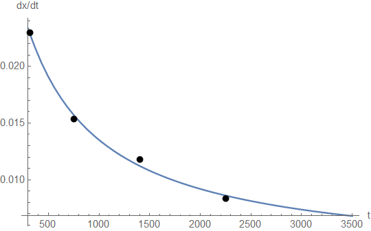
Plot[nlm[m], {m, 300, 3500}, Epilog -> {PointSize[0.02], Point@data},
 AxesLabel -> {"t", "dx/dt"}]

To get parameter table,

nlm["ParameterTable"]

Answer 2

This is simpler than Anjan Kumar's approach and gives a better fit.

t = {315, 750, 1400, 2250, 3450, 5150};
x = {10, 20, 30, 40, 50, 60};
data = Transpose[{Most[t], Differences[x]/Differences[t]}];
nlm = NonlinearModelFit[data, k (a - u)/(1 + b*u), {k, a, b}, u];
nlm["Function"][u]

-((2.00757*10^-6 (-16940.3 - u))/(1 + 0.00163761 u))

nlm["ParameterTable"]

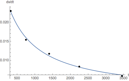
Plot[nlm[t], {t, 300, 3475},
  Epilog -> {AbsolutePointSize[5], Point[data]},
  AxesLabel -> {"t", "dx/dt"}]

Update

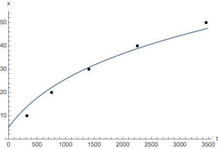
Now let's look at how this model predicts the data we started with.

xF[u_] = Integrate[nlm["Function"][u], u] + t[[1]]

0.00122591 u + 20.0188 Log[610.645 + 1. u]

However,

Table[xF[u], {u, t}] - x

{127.124, 125.369, 123.983, 122.084, 120.567, 119.652}

so xF must have a constant of integration added to it.

c = -RootMeanSquare[x - Table[xF[u], {u, t}]];
xF[u_] = xF[u] + c

-123.158 + 0.00122591 u + 20.0188 Log[610.645 + 1. u]

With[{pts = Transpose[{t, x}]},
 Plot[xF[t], {t, 0, 3475},
  PlotRange -> {Automatic, {0, 55}},
  Epilog -> {AbsolutePointSize[5], Point[pts]},
  AxesLabel -> {"t", "x"}]]