Local max/min of Mathematica data sets

Question

Is there a way in Mathematica to find the local maxima of a set of points?

Suppose you have

points={{xa,ya},{xb,yb},{xc,yc}...}

peakQ[{{x1_,y1_},{x2_,y2_},{x3_,y3_}}] := Abs[y1] > Abs[y2] && Abs[y2] < Abs[y3];
peaks=Map[#[[2]]&, Select[Partition[points,3,1],peakQ[#]&]]

Is it correct because in this way I find points but from plots I can see that I have lost some points.

Answer 1

Here s another version to do it. First: some data

points = SortBy[RandomReal[1, {50, 2}], First]

This gives you the positions of the maxima and minima:

maxima = 1 + Position[Differences[Sign[Differences[points[[All, 2]]]]], -2]
minima = 1 + Position[Differences[Sign[Differences[points[[All, 2]]]]], 2]

peaks = Extract[points,maxima]

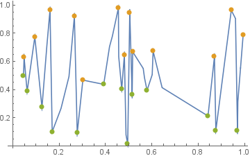
which you can see by plotting them:

ListLinePlot[points, Prolog -> {PointSize[Large], Red, Point[Extract[points, maxima]], Green, Point[Extract[points, minima]]}]

How it works:

• points[[All,2]] only takes the y-values

• Sign[Differences[...]] takes the consecutive difference, and their Sign (i.e. -1, 0, or 1)

• You are looking for something that goes up (+1) and down again (-1). So, we take Differences[...] again, and then look where the result is -2 (for maxima), or, equivalently, 2 (for minima). That is done with Position[...,2].

• We have to add 1 because taking Differences makes the lists shorter

• Extract[points,maxima] then gives you your results

And yet another version:

peaks = Pick[points[[2 ;; -2]], Differences[Sign[Differences[points[[All, 2]]]]], -2]

...with the same rationale as above, but using the functionality of Pick. One needs to drop the first and the last entry of points so that it has the same length as the other list.

Timing comparisons:

points = SortBy[RandomReal[1, {10^6, 2}], First];

peakQ[{{x1_, y1_}, {x2_, y2_}, {x3_, y3_}}] := y1 < y2 && y2 > y3
Timing[peaks1 = Select[Partition[points, 3, 1], peakQ][[All, 2]];]
(* 4 sec *)
Timing[peaks2 = Extract[points, 1 + Position[Differences[Sign[Differences[points[[All, 2]]]]], -2]];]
(* 0.4 sec *)
Timing[peaks3 = Pick[points[[2 ;; -2]], Differences[Sign[Differences[points[[All, 2]]]]], -2];]
(* 0.1 sec *)

peaks1 == peaks2 == peaks3
(* True *)

Answer 2

You can do a search for extrema (differential calculus), on the interpolated version of your dataset. See how to get an interpolated function from a set of data points here. The simplest way (assuming you have polynomial data) is to do a polynomial fit over points:

points = {
 {-5., 365.}, {-4.951, 356.571}, {-4.804, 331.998}, {-1.888, 38.604},
 {-0.018, -0.033}, {2.565, 54.056}, {3.285, 79.016}, {6.3, 159.451},
 {6.459, 160.646}, {6.715, 161.555}, {6.839, 161.524}, {7.06, 160.659},
 {8.971, 100.783}, {10.901, -85.324}, {15., -1095.}
 }; (* points sampled from -x^3 + 10 x^2 + 2 x *)

fit = Fit[points, {1, x, x^2, x^3}, x];
f = Function[{x}, Evaluate@fit]

f[x]

0.00401351 + 2.00137 x + 9.99945 x^2 - 0.999973 x^3

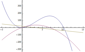
Afterwards, you can get the derivative of your curve, f. The function f is our fitted polynomial function:

Plot[{f[x], f'[x], f''[x]}, {x, -5, 15}]

Where the first derivative is zero the function has a stationary point:

sol = NSolve[{f'[x] == 0}, x, Reals]

{{x -> -0.0986535}, {x -> 6.76506}}

Checking the second derivative tells whether at the given point of interest f has a minimum or maximum (or f[x] is an inflection point):

f''[x] /. sol

{20.5912, -20.5912}

where:

• $f^{\prime\prime}(x) < 0$ -> $f$ has a local maximum at $x$.
• $f^{\prime\prime}(x) > 0$ -> $f$ has a local minimum at $x$.
• $f^{\prime\prime}(x) = 0$ -> $f$ has an inflection point at $x$

Thus:

minmax = MapThread[# -> 
   Which[#2 < 0, "max", #2 > 0, "min", True, "inflection"] &, {x /. 
   sol, f''[x] /. sol}]

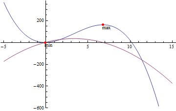
{-0.0986535 -> "min", 6.76506 -> "max"}

Plot[{f[x], f'[x]}, {x, -5, 15}, 
 Epilog -> {AbsolutePointSize@5, Red, 
   Point[{#, f[#]} & /@ (x /. sol)], Black, 
   Text[Last@#, {First@#, f@First@#}, {-1, 1}] & /@ minmax}]

Answer 3

In versions 10+, you can use FindPeaks:

SeedRandom[123]
points = SortBy[RandomReal[1, {40, 2}], First];

xvalues = MapIndexed[#2[[1]] -> #[[1]] &, points, 1];
peaks = {# /. xvalues, #2} & @@@ FindPeaks[points[[All, 2]], 0, 0, -Infinity];
valleys = {# /. xvalues, -#2} & @@@ FindPeaks[-points[[All, 2]], 0, 0, -Infinity];

ListPlot[{points, peaks, valleys}, Joined -> {True, False, False}, 
  BaseStyle -> PointSize[Large]] 

Answer 4

A solution based on code from giacomo's question, assuming that points have distinct $x$-coordinates.

In[1]:= points=SortBy[RandomReal[1,{10,2}],First]
Out[1]= {{0.0120925,0.643074},{0.180014,0.667626},{0.250923,0.696545},{0.332885,0.0217103},{0.374107,0.13732},{0.444013,0.0420624},{0.45527,0.706021},{0.547433,0.454037},{0.852822,0.897056},{0.903773,0.112657}}

As Sjoerd pointed out, we do not need to use Abs. I think you need to switch the inequalities if you want the local maximum points.

In[2]:= peakQ[{{x1_,y1_},{x2_,y2_},{x3_,y3_}}]:=y1<y2 && y2>y3

We can simply use peakQ as opposed to peakQ[#]& in Select.

In[3]:= peaks=Select[Partition[points,3,1],peakQ][[All,2]]
Out[3]= {{0.250923,0.696545},{0.374107,0.13732},{0.45527,0.706021},{0.852822,0.897056}}

Answer 5

You may use FindPeaks or PeakDetect. The parameters of each of these can be adjusted for peak selection sensitivity. Below I show with default sensitivity.

FindPeaks for TimeSeries data

First generate some data in a TimeSeries.

SeedRandom[87];
rp = RandomFunction[WienerProcess[], {0, 100, 1}];

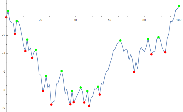
The with FindPeaks

Show[
 ListLinePlot[rp],
 ListPlot[FindPeaks[rp]["Path"], PlotStyle -> Green],
 ListPlot[(-FindPeaks[-rp])["Path"], PlotStyle -> Red]
 ]

PeakDetect for List data

data = rp["Path"];

Then

Show[
 ListLinePlot[rp],
 ListPlot[Pick[data, PeakDetect[data[[All, 2]]], 1], PlotStyle -> Green],
 ListPlot[Pick[data, PeakDetect[-data[[All, 2]]], 1], PlotStyle -> Red]
 ]

As you can see both methods select the same locations with default settings and the both have the same parameters available for adjusting selection sensitivity.

Hope this helps.