6
$\begingroup$

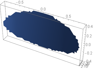
What's the preferred way to paint spots on a curved surface without getting raggedy edges? Using ParametricPlot3D with RegionFunction gets the shape I want but increasing PlotPoints slows things down considerably. Counterintuitively Reducing PlotPoints to 50 gives better looking results than 100:

With[{a = 0.8, b = 0.4, r = 5^0.5, l = 10, points = 50}, 
 ParametricPlot3D[{{x, -Sqrt[r^2 - x^2], z}, {x, Sqrt[r^2 - x^2], 
    z}}, {x, -r, r}, {z, -l/2, l/2}, 
  RegionFunction -> 
   Function[{x, y, z}, (x/a)^2 + (z/b)^2 < 1 && y > 0], Mesh -> None, 
  PerformanceGoal -> "Quality", PlotPoints -> points]]

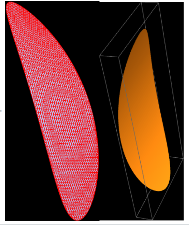
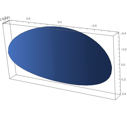
First image has points =50, second image has points = 100.

enter image description here enter image description here

$\endgroup$
2
  • 1
    $\begingroup$ The problem is that you're asking Mathematica to draw a very large plot and then throw away most of it: i.sstatic.net/YSbcF.png Why not reduce the range of x and z? With ParametricPlot3D[..., {x, -a, a}, {z, -b, b}, ...] I get a very nice plot. $\endgroup$
    – user484
    Commented Oct 29, 2016 at 17:19
  • $\begingroup$ MaxRecursion is more important here, set MaxRecursion -> 10 $\endgroup$
    – chyanog
    Commented May 17, 2022 at 6:14

4 Answers 4

3
$\begingroup$

What's the preferred way to paint spots on a curved surface without getting raggedy edges?

I use MeshFunctions, MeshShading, and Mesh:

Show[
 (* Head *)
 ParametricPlot3D[
  (1 + 0.05 Cos[u]) {Sin[u] Cos[v], Sin[u] Sin[v], 0} + {0, 0, 1.05 Cos[u]},
  {u, 0, π}, {v, 0, 2 π},
  (* mouth *)
  MeshFunctions -> {Function[{x, y, z, u, v}, x + 0.5 (2 y^2 - 2 (z + 0.5))^2]},
  MeshShading -> {Black, Lighter@Red, Yellow},
  Mesh -> {{-0.85, -0.82}},
  (*****)
  AxesLabel -> {"x", "y", "z"}, PlotPoints -> 100],
 (* Eyes *)
 ParametricPlot3D[
  Sin[1.9 (u - 0.45)]^2 (0.36 + 0.8 (Sqrt[0.5 + 2 Abs[v]])) Cos[1.5 v] *
     {-Sin[u] Cos[v], -Sin[u] Sin[v], Cos[u]},
  {u, π/6, π/2}, {v, -π/6, π/6},
  (* pupil & iris *)
  MeshFunctions -> {Function[{x, y, z, u, v}, 
     Sin[1.9 (u - 0.49)]^2 (0.36 + 0.8 (Sqrt[0.5 + 2 Abs[v]])) Cos[1.5 v]]},
  MeshShading -> {White, Lighter@Blue, Black},
  Mesh -> {{1.06, 1.077}},
  (*****)
  AxesLabel -> {"x", "y", "z"}, PlotPoints -> 100],
 (* Tongue *)
 ParametricPlot3D[
  {-u, 0, -u^2/4 - 0.15} + 0.15 Sqrt[Sqrt[(1.2 - u)]] *
     (2 Cos[v] {0, 1, 0} + Sin[v] {-u/2, 0, 1 - 0.5 Sin[v]}/Sqrt[u^2 + 1]),
  {u, 0.5, 1.2}, {v, 0, 2 π}, PlotStyle -> Red, Mesh -> None],
 PlotRange -> All
 ]
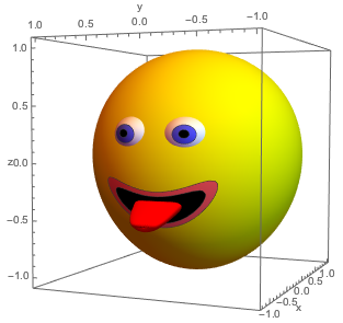
Mathematica graphics

It has the advantage of having borders that meet each other exactly. (Pasting a surface patch on another surface usually requires a small gap between them, or rounding error in the GPU causes the image to shimmer.)

$\endgroup$
2
  • 1
    $\begingroup$ +1 seems insufficient...beautiful use of mesh functions and mesh shading... $\endgroup$
    – ubpdqn
    Commented Nov 1, 2016 at 2:57
  • $\begingroup$ @"Michael E2" Nice. MeshFunctions makes more sense here than RegionFunction as I expect it defines the boundary before constructing the shape so probably reduces the calculation. I wish I had got to this before Halloween, the possibilities are endless :o) Also the comment about having the borders meet each other exactly is huge. I had needed to include a small gap just for that reason before. Your post should be part of the manual! $\endgroup$
    – DrBubbles
    Commented Nov 2, 2016 at 21:08
4
$\begingroup$

Perhaps this can achieve the desired outcome (or at least a starting point):

r = ImplicitRegion[
  x^2 + y^2 == 5 && (x/0.8)^2 + (z/0.4)^2 < 1, {{x, -5, 5}, {y, 0, 
    5}, {z, -5, 5}}]
dr = DiscretizeRegion[r, MeshCellStyle -> {1 -> Red, 2 -> Red}, 
   Background -> Black];
rp = RegionPlot3D[dr, Background -> Black];
Row[{dr, rp}]

enter image description here

$\endgroup$
2
  • $\begingroup$ nice solution, with lots of new lessons in it for me! I found however that I was able to make the shapes smooth after searching more in stackexchange and coming across suggestions to use ContourPlot3D instead of ParametricPlot3D. This worked really well, but I'm glad I got your reply first as it illustrates some new techniques for me. $\endgroup$
    – DrBubbles
    Commented Oct 21, 2016 at 6:57
  • 1
    $\begingroup$ @DrBubbles glad you found what you needed :). MMA is very flexible and I learn a lot from the creativity of this community. $\endgroup$
    – ubpdqn
    Commented Oct 21, 2016 at 7:00
4
$\begingroup$

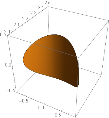
Here's a solution using ContourPlot3D:

With[{a = 0.8, b = 0.4, r = 5^0.5, l = 10}, 
 ContourPlot3D[
  x^2/r^2 + y^2/r^2 == 1, {x, -r, r}, {y, -r, r}, {z, -l/2, l/2}, 
  RegionFunction -> 
   Function[{x, y, z}, (x/a)^2 + (z/b)^2 < 1 && y > 0], Mesh -> None, 
  PerformanceGoal -> "Quality", 
  PlotRange -> {{-.9, .9}, {2, 2.5}, {-0.5, 0.5}}, PlotPoints -> 60]]

enter image description here

$\endgroup$
1
$\begingroup$

Another way:

With[{a = 0.8, b = 0.4, r = 5^0.5, l = 10, points = 75}, 
 ParametricPlot3D[{{0, r, 0}, {x, Sqrt[r^2 - x^2], z}},
  {x, -r, r}, {z, -l/2, l/2}, 
  MeshFunctions -> {Function[{x, y, z, s, t}, (x/a)^2 + (z/b)^2]}, 
  Mesh -> {{1}}, MeshShading -> {Automatic, None}, 
  PerformanceGoal -> "Quality", PlotPoints -> points, 
  PlotRange -> All]]

Mathematica graphics

$\endgroup$

Your Answer

By clicking “Post Your Answer”, you agree to our terms of service and acknowledge you have read our privacy policy.

Not the answer you're looking for? Browse other questions tagged or ask your own question.