Calculating the error in the solution of a system of ODEs

Question

I have solved system of ODEs by using NDSolve. I want to calculate the error of the solutions. So far I have calculated error by plotting results of each equation.

1. Is what I'm doing the correct way to obtain the error for my problem?
2. I am not sure the results I am getting are accurate enough. If not, then kindly suggest some other way to calculate the error.

My code for solving the system of ODEs

s = 
  NDSolve[
    {x''[t] == -(1/2)*y[t]*x'[t], y''[t] == x'[t], 
     x'[0] == -1 + x[0], y[0] == 0, x[10] == 0, y'[10] == 0}, 
    {x, y}, {t, 20}]

I am examining the error for the 1st equation with

Plot[(x''[t] + (1/2)*y[t]*x'[t]) /. s, {t, 1, 10}, WorkingPrecision -> 50]

and for the 2nd equation

Plot[(y''[t] + x'[t]) /. s, {t, 1, 10}, WorkingPrecision -> 50]

Answer 1

There are two sources of error to investigate, the error in the steps and the interpolation error.

First, to explore the error, I usually set up some variables to make it easier:

ode = {x''[t] == -(1/2)*y[t]*x'[t], y''[t] == x'[t]};
bcs = {x'[0] == -1 + x[0], y[0] == 0, x[10] == 0, y'[10] == 0};
residuals = ode /. Equal -> Subtract;
{s} = NDSolve[{ode, bcs}, {x, y}, {t, 20}]

I separate the ode from the initial/boundary conditions bcs. The residuals can be computed directly from ode, which prevents transcription errors and maintenance errors if ode is changed.

[Side note: The assignment {s} = NDSolve[..] is my peculiarity. Its purpose is to perform a simple check on the solution. See end for discussion.]

We can use ListPlot/ListLogPlot to plot the steps and Plot/LogPlot for the interpolating functions. I usually use a log-plot because the error often exhibits a range of several orders of magnitude. I sometimes use a regular plot of RealExponent[residuals], which is equivalent to a log-plot of Abs[residuals].

Error at the steps

The times of the steps can be obtained with either of these:

x["Coordinates"] /. s
x["Grid"] /. s

They are structured lists. To get flat list of the times, use Flatten. [Note that for a PDE, which has a domain of more than one dimension, these lists are structured differently, and you cannot simply use Flatten.]

The code

residuals /. t -> x["Coordinates"] /. s

first replaces t by a list {{t1, t2,...}}, and then replaces x and y by their InterpolatingFunction solutions. This works because InterpolatingFunction threads over lists as do the basic arithmetic operations. Thus the following yields a plot of the residuals at the steps by step number.

ListPlot[
 RealExponent[Flatten /@ (residuals /. t -> x["Coordinates"] /. s)],
 Frame -> True]

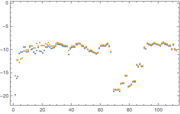
If you want to plot the residuals versus t, it's somewhat somewhat simpler to process each residual separately and list the ordered pairs using Table:

With[{data = {
    Table[{t, Abs@residuals[[1]]} /. s, {t, x["Coordinates"] /. s // Flatten}],
    Table[{t, Abs@residuals[[2]]} /. s, {t, x["Coordinates"] /. s // Flatten}]}},
 ListLogPlot[
  data,
  Frame -> True, PlotRange -> All]
 ]

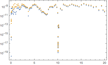
The plot could be done with RealExponent and ListPlot as in the previous one, but I thought I'd show the variant with LogPlot and Abs.
The spike at t == 10 is probably due to NDSolve choosing t == 10 as the starting time for the initial condition in the shooting method it uses to solve the BVP.

Error of the interpolation

Dealing with the interpolations is easier. What we see below is that the error between the steps is greater. Plotting with some transparency makes it easier to examine both residuals.

Plot[RealExponent[residuals /. s] // Evaluate,
 {t, 0, 20}, PlotStyle -> Opacity[0.75], Frame -> True]

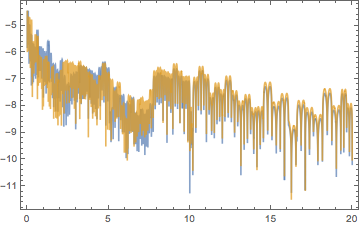
The deep spikes between the steps are typical of Hermite cubic interpolation. The plot below is typical of the residuals between steps:

With[{step = 100},
 Plot[residuals /. s // Evaluate, 
  Evaluate@Flatten[{t, (x["Grid"] /. s)[[{step, step + 1}]]}], 
  PlotStyle -> Opacity[0.75], Frame -> True]]

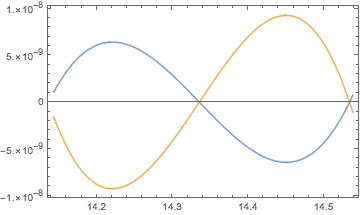
One can infer that the spikes are where each residual crosses zero, as well as smaller ones at the steps themselves (all of which may by limited by the resolution of the plot).

Improving the error

By default, NDSolve usually returns a Hermite piecewise cubic interpolation of the steps

{sALL} = NDSolve[{ode, ics},    (* same solution as `s`, but with "dense output" *)
  {x, y}, {t, 20}, 
  InterpolationOrder -> All]

{sRK} = NDSolve[{ode, ics},      (* different method, for the sake of comparison *)
  {x, y}, {t, 20}, 
  Method -> "ExplicitRungeKutta", InterpolationOrder -> All]

From below, one can see that the dense outputs take much more memory, even though sALL has the same steps as s and sRK has many fewer steps.

Length /@ (x["Grid"] /. {s, sALL, sRK})  (* number of steps *)
ByteCount /@ {s, sALL, sRK}              (* memory used by the solution *)
(*
  {112, 112, 37}
  {12024, 153352, 70024}
*)

The three solution use three different methods of interpolation.

x["InterpolationMethod"] /. {s, sALL, sRK}
(*  {"Hermite", "Local Taylor series", "Chebyshev"}  *)

If you look at the error at the steps as above, you will see that for s and sALL, they are exactly the same. The error for sRK turns out to be much better, but it's using a different method. What's more important is that the dense output solutions have much less error between the steps.

Plot[
 Join[
   RealExponent[residuals /. s],
   RealExponent[residuals /. sALL],
   RealExponent[residuals /. sRK]] // Evaluate,
 {t, 0, 20},
 PlotStyle ->
  {Opacity[0.4], Opacity[0.4], Opacity[0.6], Opacity[0.6], Opacity[0.8], Opacity[0.8]},
 PlotLegends -> {"s[[1]]", "s[[2]]", "sALL[[1]]", "sALL[[2]]", "sRK[[1]]", "sRK[[2]]"},
 Epilog -> {Red, Point@Thread[{Flatten[x@"Grid" /. sRK], -17}]}
 ]

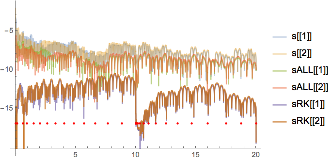
One can see that the residuals for sALL are about two orders of magnitude small. For sRK, they are much smaller than that. Note for sRK there are several spikes between each step. This is typical of collocation methods, which interpolate the ode at several points; the solution is based on the corresponding interpolating polynomial. The residual at a typical step may look like this:

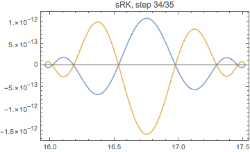
One can see that the dense output improves accuracy considerably. The question each user has to answer, is what accuracy is sufficient? When is the dense output worth it?

Checking NDSolve's notion of error

Mathematica has a somewhat more complicated measure of error to handle the fact that as a solution gets closer to zero it gets harder to achieve a PrecisionGoal; in such circumstance, the AccuracyGoal becomes dominant. See the tutorial Norms in NDSolve.

The error norm is scaled so that a value below one indicates that the PrecisionGoal and AccuracyGoal have been met.

svn = NDSolve`ScaledVectorNorm[Infinity, 10.^(-MachinePrecision/2) {1, 1}];
Max@ Map[
 svn[residuals,
     {x''[t], y''[t]} /. First@Solve[ode, {x''[t], y''[t]}]] /. s /. t -> # &, 
 Flatten[x["Coordinates"] /. s]
 ]
(*  0.467073  *)

So the worst step is comfortably within the margin of error.

---

[Re: The assignment {s} = NDSolve[..]. It performs a simple check on the solution. NDSolve returns a list of solutions, the length of which list depends on the degree of the system (of the highest order derivatives). Note each solution is itself a list of functions for each dependent variable. For a quasilinear system such as ode in the OP's case, the number of solutions will be 1. An assignment of the form {s} = NDSolve[..] will fail if the ode is not quasilinear or if NDSolve fails. The examples in the document apply First, either to First[s] if s = NDSolve[..], or s = First@NDSolve[..]. Such code does not fail if ode has multiple solutions; instead, it throws away any solutions after the first. To unwittingly throw them away is a serious error, which {s} = NDSolve[..] detects. The annoying thing about my way is that when there are multiple solutions, they are discarded, although they can be retrieved with %, if $HistoryLength is greater than zero. Another way that preserves a multiple solution would be the assignments {s} = s = NDSolve[..]. But sometimes I only want to overwrite s if NDSolve returns a solution.]