Issuing with ParametricNDSolveValue

Question

I am having a problem with ParametricNDSolveValue[] . let me start with a simple example. Considered following example with constant parameter $a$.

pfun = ParametricNDSolveValue[{y'[x] == y[x] Cos[x + y[x]], 
   y[0] == a}, y, {x, 0, 30}, {a}]

Plot the solutions for several different values of the parameter gives:

Plot[Evaluate[Table[pfun[a][t], {a, -1, 1, .1}]], {t, 0, 1}, 
 PlotRange -> All]

Now, consider the following case:

pfun = ParametricNDSolveValue[{y'[x] == y[x] Cos[x + y[x]], 
   y[a] == 1}, y, {x, 0, 30}, {a}] 

and trying to plot the function I end up with following error "Cannot find starting value for the variable".

Plot[Evaluate[Table[pfun[a][t], {a, -1, 1, .1}]], {t, 0, 1}, 
 PlotRange -> All]

ParametricNDSolveValue::ndsv: Cannot find starting value for the variable y. >>    
ParametricNDSolveValue::ndsv: Cannot find starting value for the variable y. >>    
ParametricNDSolveValue::ndsv: Cannot find starting value for the variable y. >>    
General::stop: Further output of ParametricNDSolveValue::ndsv will be suppressed during this calculation. >>

I will appreciate for any solution.

Answer 1

As you have noted placing the parameter on the left hand side of a boundary condition:

y[b] == 1

does not work. You are forced to keep the parameter on the right hand side.

y[0] == a

What can be done is to keep the parameter on the RHS and then use numerical methods to determine the value of b for a particular a parameter (in other words, seek a relationship between a and b).

First solve the ParametricNDSolveValue using a as the parameter.

pfunRHS = ParametricNDSolveValue[
  {
   y'[x] == y[x] Cos[x + y[x]],
   y[0] == a
   },
  y,
  {x, 0, 30},
  {a}
  ]

Next, define a function that produces a number when given a parameter value and an x coordinate.

y[x_?NumericQ, a_?NumericQ] := Evaluate[pfunRHS][a][x]

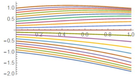
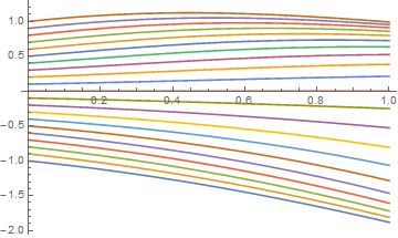
Here is a plot in the interval zero to one for various a values.

Plot[Evaluate[Table[y[t, a], {a, -1, 1, .1}]], {t, 0, 1}, 
 PlotRange -> All]

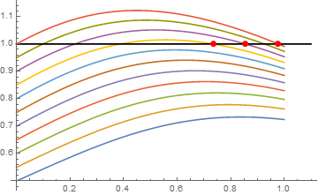
What we have to do is select a value for the a parameter and than solve for the corresponding b value where y[b,a]=1. Graphically this is where the black line intersects equal contours of a.

Show[
 Plot[Evaluate[Table[y[t, a],
    {a, 0.5, 1, .05}]], {t, 0, 1},
  PlotRange -> All],
 ListLinePlot[{{0, 1}, {1.1, 1}},
  PlotStyle -> Black]
 ]

Note that below a certain a parameter threshold (approximately 0.85) there is no solution.

Given an a we can use FindRoot to determine the corresponding b. Here are two values.

FindRoot[
 {
  a - 1,
  y[b, a] - 1
  },
 {{a, 1}, {b, 0.8}}
 ]
(* {a -> 1., b -> 0.978505} *)

FindRoot[
  {a - 0.9,
   y[b, a] - 1
   },
  {{a, 1}, {b, 0.8}}
  ]
(* {a -> 0.9, b -> 0.855604} *)

If one tries a = 0.8 you get an error.

About the lowest one can go is 0.85 for a.

FindRoot[
 {a - 0.85,
  y[b, a] - 1
  },
 {{a, 0.85}, {b, 0.8}}
 ]
(* {a -> 0.85, b -> 0.735357} *)

Superimpose the three points on the plot

Show[
 Plot[Evaluate[Table[y[t, a], {a, 0.5, 1, .05}]], {t, 0, 1}, 
  PlotRange -> All],
 ListLinePlot[{{0, 1}, {1.1, 1}}, PlotStyle -> Black],
 ListPlot[{{0.975, 1}, {0.8556, 1}, {0.735357, 1}},
  PlotStyle -> {PointSize -> Large, Red}]
 ]

Create a function to retrieve the b value given an a value.

getB[aStart_?NumericQ] := Module[
  {
   sol
   },
  sol = FindRoot[
    {a - aStart,
     y[b, a] - 1
     },
    {{a, aStart}, {b, 0.8}}
    ];
  sol[[2, 2]]
  ]

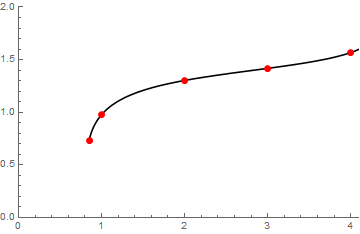
Plot b vs a

Show[
 Plot[getB[a], {a, 0.85, 5},
  PlotStyle -> Black,
  PlotRange -> {{0, 4.1}, {0, 2}}
  ],
 ListPlot[{
   {0.85, getB[0.85]}, {1, getB[1]},
   {2, getB[2]}, {3, getB[3]}, {4, getB[4]}
   },
  PlotStyle -> {PointSize -> Large, Red}]
 ]

I didn't want to introduce a diversion but the range of a that works has an upper limit as well, around 4.

It may be, depending upon your actual problem, you may be able to develop a functional relationship between a and b from the numerical results.