2
$\begingroup$

This question is a follow-up to a previous question.

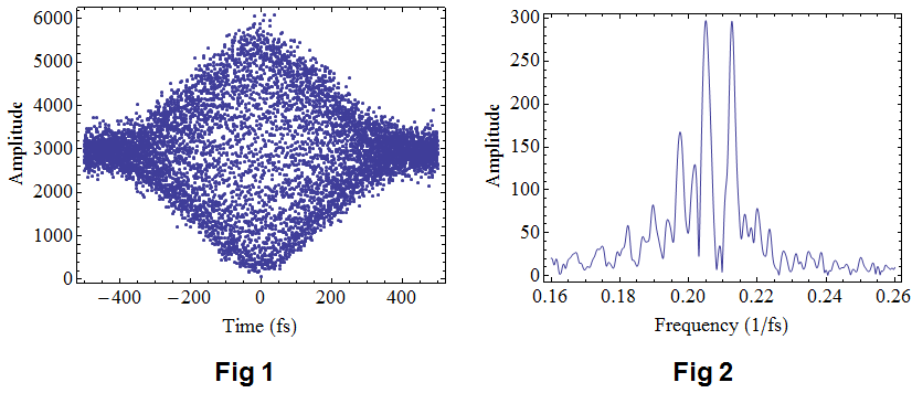
I need to perform a Fourier Transformation on an experimental data in time-domain, as shown in Fig 1. With the kind help from Daniel Lichtblau and BlacKow, I have already obtained the spectral distribution (in Fig 2) of this time-domain data. enter image description here
The codes are shown below

    SetDirectory[NotebookDirectory[]];
    name = "try.txt";
    a = Import[name, "Table"];
    ListLinePlot[a, PlotRange -> All, Joined -> False, Mesh -> Full, Axes -> False, Frame -> True, AspectRatio -> .75,  LabelStyle -> Directive[Black, FontSize -> 18],  FrameLabel -> {{"Amplitude", None}, {"Time (fs)", None}},  ImageSize -> {400, 300}]

    data = a;
    {times, vals} = Transpose[data];
    IFT[(w_)?NumberQ, vals_, times_] :=  Total[vals*Exp[(-I)*2 \[Pi]*w*times]]/Length[times]; 
    Plot[Abs[IFT[w, vals, times]], {w, 0.16, 0.26}, PlotRange -> All,  Frame -> True, Axes -> False,  LabelStyle -> Directive[Black, FontSize -> 18], AspectRatio -> .75,  FrameLabel -> {{"Amplitude", None}, {"Frequency (1/fs)", None}},  ImageSize -> {400, 300}]

The problem is that the spectral distribution in Fig 2 is a little far away from my theoretical expectation, which should be a Gaussian-like distribution, according to my experimental condition. But Fig 2 has too many peaks, not a single-peak Gaussian-like distribution.

The multi-peak distribution in Fig 2 may be caused by the imperfection in the experiment. Fig 3 is an enlarged figure of Fig 1. In Fig 3, the red curve corresponds to a fitting function of the experimental blue dots. If everything is perfect, the sampling period should be the same. But due to the unstable condition of the scanning Piezo in experiment, the sampling period was changing all the time, as shown in Fig 3. It was hard to calibrate the condition of the Piezo.

enter image description here

The codes for Fig 3 are:

    Show[ListPlot[a, PlotRange -> {{0, 200}, All}], Plot[2931.8 + 11000/3 E^(-(t^2/45000)) Sqrt[2/\[Pi]] Cos[25/66 \[Pi] (-2.0314 + t)], {t, 0, 200}, PlotStyle -> {Red},   PlotRange -> All], Axes -> False, Frame -> True, AspectRatio -> .2,  FrameLabel -> {"Time (fs)", "Intensity"}, LabelStyle -> Directive[Black, FontSize -> 18],  ImageSize -> {1000, 200}] 

My dream is to remove the multi-peak structure (frequency noises) in Fig 2, and obtain a single peak in a Gaussian-like distribution. Is it possible to remove the frequency noises? Any suggestion or help will be highly appreciated.

$\endgroup$
2
  • $\begingroup$ Why do you have such dream? If you know for sure that there should be only one peak, then you only need to fid its frequency. In this case @JasonB's solution is the perfect way of doing it. $\endgroup$
    – BlacKow
    Commented Apr 4, 2016 at 16:46
  • $\begingroup$ @BlacKow. According to my theoretical expectations, there should be only one peak. But I need to prove this using the experimental raw data, not only by theoretical assumption. However, there are too many noise in the data. $\endgroup$
    – user14634
    Commented Apr 5, 2016 at 4:17

1 Answer 1

4
$\begingroup$

It is possible, but I don't know that this method is desirable. I notice from your data that the signal doesn't decay to zero at the endpoints, which can lead to a lot of shoulder peaks across the spectrum. You can apply a windowing function to the data prior to taking the Fourier transform, which will have the effect of smoothing the shoulder peaks and of broadening the main peak.

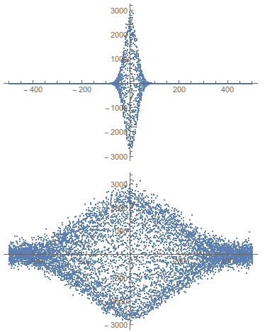
Here is the windowed versus original data,

window = (Exp[-#^2/(2 25.0^2)]) & /@ times;
ListPlot[Transpose[{times, (vals - Mean@vals) window}], 
 PlotRange -> All]
ListPlot[Transpose[{times, (vals - Mean@vals)}] , PlotRange -> All]

enter image description here

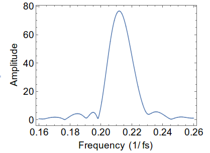
And here is the transform of the windowed data, modifying the code above via

IFT[(w_)?NumberQ, vals_, times_] := 
  Total[((vals - Mean@vals) window)*Exp[(-I)*2 \[Pi]*w*times]]/
   Length[times];

enter image description here

I don't see how to get a single narrow peak from the data without filtering out the undesired frequency ranges, and then you need to know beforehand where the peak should be.

$\endgroup$
9
  • $\begingroup$ Thanks a lot again for your kind help. Your method of adding a window really suppressed the multi-peak. But, this window is too small and raw data was partially changed. The bandwidth information is the most important information for me. Is it possible to design a bigger window such that the raw data is changed as few as possible? $\endgroup$
    – user14634
    Commented Apr 5, 2016 at 4:25
  • $\begingroup$ @user14634 - I think that is specifically not possible. That is, with this data, it is not possible to extract a single frequency and bandwidth. In your post you said you wanted a single peak, and the only way to do that with this data, to my knowledge, is to apply the window and broaden the two peaks such that they merge. $\endgroup$
    – Jason B.
    Commented Apr 5, 2016 at 6:59
  • $\begingroup$ @ JasonB, I have already known the center frequency, since I can measure the center frequency in experiment by using other devices, e.g., a spectrometer. What I most want to obtain from this time-domain interference data, is the bandwidth, i.e., the time-domain width and the frequency-domain width (after Fourier transform). $\endgroup$
    – user14634
    Commented Apr 5, 2016 at 9:30
  • $\begingroup$ @user14634 and is that center frequency in the center of the two peaks you get above? $\endgroup$
    – Jason B.
    Commented Apr 5, 2016 at 9:31
  • $\begingroup$ @ JasonB, Yes, the frequency center should be 0.2124. $\endgroup$
    – user14634
    Commented Apr 5, 2016 at 9:53

Your Answer

By clicking “Post Your Answer”, you agree to our terms of service and acknowledge you have read our privacy policy.

Not the answer you're looking for? Browse other questions tagged or ask your own question.