4
$\begingroup$

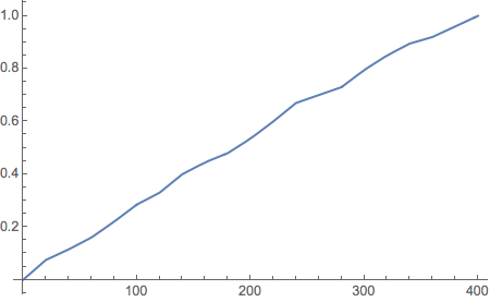
I have about 200 real numbers spread over the range 0-400. I use HistogramDistribution to bin them and PDF to create the resulting step-wise probability distribution. I assumed that CDF applied to the HistogramDistribution would yield a continuous, piece-wise linear function, but I keep getting these annoying gaps in the plot of the CDF.

Here's the code I'm using applied to some random data:

data = Table[400*RandomReal[], {200}];
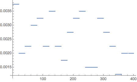
pd = PDF[HistogramDistribution[data, 20]];
Plot[pd[x], {x, 0, 400}]
Plot[CDF[HistogramDistribution[data, 20], x], {x, 0, 400}]

Any idea what's causing the gaps and how to get rid of them?

$\endgroup$
4
  • 3
    $\begingroup$ Add PlotPoints -> 500 to your final Plot command. $\endgroup$
    – bill s
    Commented Jan 25, 2016 at 3:25
  • 5
    $\begingroup$ @bills Exclusions -> None is the better approach in this case. $\endgroup$ Commented Jan 25, 2016 at 4:48
  • 1
    $\begingroup$ If your real data displays near zero values for the histogram in the extremes of the data (as opposed to data from distributions like a uniform where the density is very non-negative at the boundaries), you might consider using SmoothKernelDistribution instead. This gives you a smooth curve for the density rather than a bumpy histogram. You can use PDF and CDF with the object produced by SmoothKernelDistribution just like HistogramDistribution. $\endgroup$
    – JimB
    Commented Jan 25, 2016 at 7:32
  • 1
    $\begingroup$ Yet another option would be to use DiscretePlot with your CDF; DiscretePlot[CDF[HistogramDistribution[data, 20], x], {x, 0, 400}, Filling -> None, Joined -> True] generates this plot. As an aside, your data can be more efficiently generated using: data = RandomReal[{0, 400}, 200]. $\endgroup$
    – MarcoB
    Commented Jan 27, 2016 at 23:38

2 Answers 2

5
$\begingroup$

This answer is based on Brett Champion's comment. The gaps can be removed by giving the option Exclusions -> None.

SeedRandom[1]; data = RandomReal[400, 200];

Plot[PDF[HistogramDistribution[data, 20], x], {x, 0, 400}]

pdf

Plot[CDF[HistogramDistribution[data, 20], x], {x, 0, 400}, Exclusions -> None]

cdf

$\endgroup$
0
$\begingroup$

The discreteness imposed by the arbitrary parameters of a Histogram seems an unnecessary burden to me. I would do

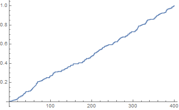
ed = EmpiricalDistribution[data];

Plot[CDF[ed, x], {x, 0, 400}, Exclusions -> None]

Mathematica graphics

with no arbitrary smoothness and discontinuities in the slope other than the one imposed by the data itself.

$\endgroup$
2
  • $\begingroup$ Unfortunately, unlike the RandomReal[400,200] example data, the real data has a low probability tail with significant gaps. I thought the histogram bins would help smooth that out a bit, giving something closer to the actual smooth distribution than the extended zero regions of an Empirical Distribution[data]. $\endgroup$ Commented Feb 15, 2016 at 14:41
  • $\begingroup$ I guess this goes beyond the Mathematica topic, but in terms of my scientific "ideology" I have little appreciation for parametric estimators, such as histograms, precisely because they allow artificial beautification of the data. Histograms perform the worse in tailed distributions and are only tolerable for almost normal distributions. $\endgroup$
    – rhermans
    Commented Feb 15, 2016 at 15:03

Not the answer you're looking for? Browse other questions tagged or ask your own question.