6
$\begingroup$

I am working on a signal processing project with two oscillators. The first oscillator has a frequency $f_1$ that is independent, and the second oscillator has a frequency $f_2$ that increases, and will become 'frequency entrained' (i.e., 'synchronized', or 'phase locked') when its near to $f_1$.

The best way to determine if the two oscillators are phase locked is to compare the phases of both signals. The real data is messy and a bit cumbersome, but a minimum working example might be two data sets like this:

phases1 = {0, 1, 2, 3, 4, 5, 6, 7, 8, 9, 10, 11, 12, 13, 14, 15, 16, 17, 18, 19, 20}
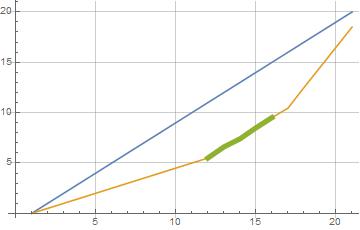
phases2 = {0., 0.5, 1., 1.5, 2., 2.5, 3., 3.5, 4., 4.5, 5., 5.5, 6.5, 7.5, 8.5, 9.5, 10.5, 12.5, 14.5, 16.5, 18.5}

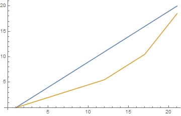
Phases of Two Oscillators

There is a spot in the middle where the two lines are parallel. One way to find where they are parallel is to take the derivative of both lists and subtract:

Differences[phases1] - Differences[phases2]

And then use a list manipulation function to locate the zeros. However, for the system I am working with, this isn't good enough because of noise and other issues. Is there a better way to determine when two lists are parallel in mathematica?

Should I use autocorrelation or some other function?

$\endgroup$
7
  • $\begingroup$ Does Differences[phases1] - Differences[phases2] work when filtering the data (for example low-pass-filter to remove some noise) to a sufficient degree? $\endgroup$
    – Sascha
    Commented Dec 23, 2015 at 20:21
  • $\begingroup$ It does identify the region where synchronization occurs, but not the whole region. It misses a significant percentage of the ends. It is important to know when the synchronization begins. $\endgroup$ Commented Dec 23, 2015 at 20:29
  • $\begingroup$ Have you tried both filtering the data and afterwards using Differences and using a Filter on the difference of the signals? $\endgroup$
    – Sascha
    Commented Dec 23, 2015 at 20:31
  • 1
    $\begingroup$ You might consider asking this question on Cross Validated as a statistical approach that treats this as a model fitting task that gives you estimates of precision for the starting and ending points of the synchronization. $\endgroup$
    – JimB
    Commented Dec 23, 2015 at 22:07
  • 1
    $\begingroup$ Without a meaningful noise estimate, we can only guess at what you're seeing. An observation: If you subtract, phases1 - phases2, the parallel segment becomes the constant segment. Detecting constant segments is, perhaps, easier to do. (It's samples 12-17.) But in the face of noise, "Where does the character of the difference trace change from rising to flat and then again from flat to falling?" cannot have a sharp answer. To make confidence claims requires a noise model and a signal model. $\endgroup$ Commented Dec 24, 2015 at 1:11

3 Answers 3

8
$\begingroup$

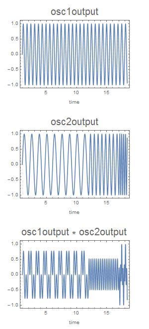
Here is the basic analog engineer approach. Multiply the outputs of your oscillators and apply a lowpass filter:

    phases1 = {0, 1, 2, 3, 4, 5, 6, 7, 8, 9, 10, 11, 12, 13, 14, 15, 16, 
  17, 18, 19, 20}
    phases2 = {0, 0.5, 1., 1.5, 2., 2.5, 3., 3.5, 4., 4.5, 5., 5.5, 6.5, 
  7.5, 8.5, 9.5, 10.5, 12.5, 14.5, 16.5, 18.5}  

k = 10; (* k = it scales the frequencies; your frequencies are certainly  
different; can be a problem *)

(* ouputs of the oscillators :*)
osc1output[t_] = 
  Sin[k Interpolation[phases1, InterpolationOrder -> 1][t]];
osc2output[t_] = 
  Sin[k Interpolation[phases2, InterpolationOrder -> 1][t]];
tfin = 18.4;

(* graphics rendering : *)
options = {Frame -> True, ImageSize -> 300, Axes -> False, 
   ImagePadding -> 40};
Column[{Plot[osc1output[t], {t, 1, tfin}, Evaluate @ options, 
   FrameLabel -> {"time", "", Style["osc1output", FontSize -> 20]}],
  Plot[osc2output[t], {t, 1, tfin}, Evaluate @ options, 
   FrameLabel -> {"time", "", Style["osc2output", FontSize -> 20]}],
  Plot[osc1output[t]* osc2output[t], {t, 1, tfin}, Evaluate @ options,
    FrameLabel -> {"time", "", 
     Style["osc1output * osc2output", FontSize -> 20]}]}, 
 Dividers -> None]

plots

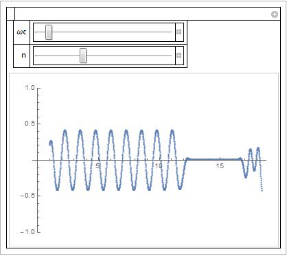
Low pass filter, adjusted a posteriori:

mySampleRate = 100; (* should be larger than your frequencies, say at least  
                       ten times *)
l1 = Table[osc1output[t] osc2output[t], {t, 1, tfin, 1./mySampleRate}];
Manipulate[
 ListPlot[LowpassFilter[l1, ωc, n, SampleRate -> mySampleRate],
   PlotRange -> {Automatic, {-1, 1}}, 
  DataRange -> {1, tfin}], {{ωc, 8.2}, 0, 100}, {{n, 139}, 0, 
  400, 1}]

Manipulate

When the frequencies are the same, the filtered signal is constant, and not necessarily zero (here, it's a coincidence).

$\endgroup$
2
  • $\begingroup$ I would certainly take the same route, but did you try with noise? $\endgroup$
    – sebhofer
    Commented Dec 24, 2015 at 9:32
  • $\begingroup$ I tried this and it works very nicely, along with a moving average. $\endgroup$ Commented Dec 26, 2015 at 21:07
5
$\begingroup$

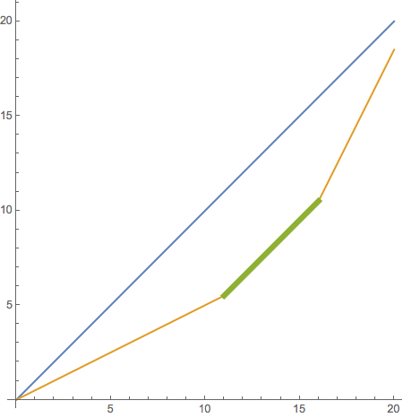
This is very similar to eldo's answer, but IMO a little more robust.

data1 = Range[0, 20];
data2 = Join[Range[0., 5.5, .5], Range[6.5, 10.5], Range[12.5, 18.5, 2.]];

getIndices[data1_, data2_, threshold_: 1.*^-3] :=
  Module[{indices},
    indices =
      MapIndexed[
        If[Abs[#1] < threshold, #2, Nothing] &, 
        Differences[Thread[Subtract[data1, data2]]]];
    Append[indices, Last[indices] + 1]]

With[{indices = getIndices[data1, data2]},
  ListLinePlot[
    {Transpose[{data1, data1}],
     Transpose[{data1, data2}],
     Transpose[{Flatten[indices] - 1, Extract[data2, indices]}]},
    AspectRatio -> Automatic,
    PlotStyle -> {Automatic, Automatic, AbsoluteThickness[5]}]]

plot

$\endgroup$
3
$\begingroup$
p1 =
  {0, 1, 2, 3, 4, 5, 6, 7, 8, 9, 10, 11, 12, 13, 14, 15, 16, 17, 18, 19, 20};

Some noise added

p2 = 
  {0., 0.5, 1., 1.5, 2., 2.5, 3., 3.5, 4., 4.5, 5., 5.5, 6.6, 7.4, 
   8.5, 9.51, 10.45, 12.5, 14.5, 16.5, 18.5};

dif = Abs[Differences@p1 - Differences@p2];

Position of differences <= n to allow for noise

pos = Position[dif, a_Real /; a <= 0.25];

"Parallel" section

p3 = Transpose[{Flatten@pos, Extract[p2, pos]}]

 ListLinePlot[{p1, p2, p3},
   GridLines -> Automatic,
   PlotStyle -> {Automatic, Automatic, [email protected]}]

enter image description here

$\endgroup$
1
  • $\begingroup$ without trying this approach I guess it only works for minimal noise (as one can see, even in the chosen example some piece of the parallel slope is left ) $\endgroup$
    – Sascha
    Commented Dec 23, 2015 at 21:20

Your Answer

By clicking “Post Your Answer”, you agree to our terms of service and acknowledge you have read our privacy policy.

Not the answer you're looking for? Browse other questions tagged or ask your own question.