10
$\begingroup$

Executing

a = PDF[TransformedDistribution[
x^2 + y^2 + z^2, {x \[Distributed] UniformDistribution[{-1, 2}], 
 y \[Distributed] UniformDistribution[{-1, 2}], 
 z \[Distributed] UniformDistribution[{-1, 2}]}], t] //AbsoluteTiming

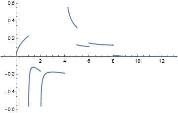
, I obtain a long output (see it here) in 5747.98 sec. The result is not correct in view of

Plot[a[[2]], {t, -1, 13}, PlotStyle -> Thick]

enter image description here

since any PDF cannot take negative values. Is there a workaround?

$\endgroup$
5
  • $\begingroup$ What it should look like for reference: dist = HistogramDistribution[ Norm[#]^2 & /@ RandomVariate[UniformDistribution[{{-1, 2}, {-1, 2}, {-1, 2}}], 10000000] , 250]; Plot[PDF[dist, t], {t, -1, 13}, PlotStyle -> Thick, Exclusions -> None, PlotRange -> All] $\endgroup$
    – flinty
    Commented Jul 28, 2021 at 9:54
  • $\begingroup$ Also worth noting that removing a dimension (e.g z) produces a correct result for 2D. $\endgroup$
    – flinty
    Commented Jul 28, 2021 at 9:59
  • $\begingroup$ @flinty: Thank you for your interest to the question. Indeed, the plot should be similar to the histgram of Norm[#]^2 & /@RandomVariate[UniformDistribution[{{-1, 2}, {-1, 2}, {-1, 2}}], 10000000]. Yes, Mathematica produces the correct result in two dimensions. $\endgroup$
    – user64494
    Commented Jul 28, 2021 at 10:39
  • $\begingroup$ The results of b = CDF[TransformedDistribution[ x^2 + y^2 + z^2, {x \[Distributed] UniformDistribution[{-1, 2}], y \[Distributed] UniformDistribution[{-1, 2}], z \[Distributed] UniformDistribution[{-1, 2}]}], t] in 10571. sec and Plot[b, {t,-1,13},PlotStyle->Thick] are even worse. $\endgroup$
    – user64494
    Commented Jul 28, 2021 at 11:37
  • 5
    $\begingroup$ If you found an obvious bug, you should report it to Wolfram Support. $\endgroup$
    – Szabolcs
    Commented Jul 29, 2021 at 8:09

2 Answers 2

17
$\begingroup$

The Issue

Mathematica appears to have a lot of trouble with doing the integrals involved in finding the PDF. I'm not sure what's going on under the hood, but doing some playing around suggests Mathematica is somehow screwing up when it comes to the degeneracies involved with having a non-symmetric interval involving both positive and negative numbers. E.g. in 1D the PDF of $A=X^2$ with $X\sim U(-1,2)$ is given by $$ f_A(a)=\begin{cases} \frac{1}{3 \sqrt{a}} & 0<a<1 \\ \frac{1}{6 \sqrt{a}} & 1<a<4\\ 0&\text{else} \end{cases} $$ which is discontinuous because $0<a<1$ get contributions both from when $-1<x\leq0$ and $0<x<1$ while $1<a<4$ get contributions only from $1<x<2$. Mathematica has no problem handling this in 1D. In 2D, these degenerate contributions become more complex but Mathematica still gets it right. However, in 3D it seems Mathematica no longer handles these degeneracies correctly. This may be caused by the fact that Mathematica has to resort to different techniques in 3D because it cannot evaluate the integrals in the same way. I ran into some of this playing around with using the direct formula for the transformation. Naively applying it works in 2D but not 3D. Doing some change of variables stuff (e.g. $w=a-x^2$) gives integrals of the form$^1$ $$ f_A(a)=\int _{a-b}^{a-c}\int _{w-d}^{w-e}\int _{v-f}^{v-g}\frac{\delta (k) dkdvdw}{8 \sqrt{v-k} \sqrt{w-v} \sqrt{a-w}} $$ which Mathematica can do in 2D (same form with one less $\sqrt{\cdot}$ and integral) but not 3D, for all values of $b-g\in\{0,1,4\}$.

Whatever the underlying reason, here's an example of where Mathematica gets it wrong and how we can work around that. Consider the CDF in 3D for $1<a<2$

Integrate[Boole[x^2+y^2+z^2<= a], 
{x,y,z} ∈ Cuboid[{-1,-1,-1},{2,2,2}], Assumptions-> 1<a<2]/3^3/. a-> 3/2

gives $\sim 0.045$ but the correct answer is $\sim 0.265$ and can be found by handling the cases separately:

{r1,r2}={Cuboid[{-1,-1,-1},{1,1,1}],Cuboid[{-1,-1,1},{1,1,2}]};
(Integrate[Boole[x^2+y^2+z^2<= a], {x,y,z} ∈ r1, Assumptions-> 1<a<2]+
3 Integrate[Boole[x^2+y^2+z^2<= a], {x,y,z} ∈ r2, Assumptions-> 1<a<2])/3^3/. a-> 3/2

Which comes from the fact that for $1<a<2$ the magnitude of $x$, $y$, and $z$ are all $\leq1$ or two are $\leq1$ and one is $>1$. The factor of three arises because any one of the three $x$, $y$, or $z$ can be the one which is $>1$. This motivates our workaround.

A workaround

We handle the cases manually for Mathematica, what's given here should work well in any dimension (though some tweaking would need to be done). We need to consider the following regions and multiplicities

dim=3
b3 = Union[Tuples[{{-1, 1}, {1, 2}}, dim], SameTest -> (Sort[#1] == Sort[#2] &)];
regs = Cuboid @@ Thread[#] & /@ b3;
mult = Length@Permutations[#] & /@ b3;

We then define the integral for the CDF

int[as_]:=int[as]=mult.(ParallelMap[Integrate[Boole[x^2+y^2+z^2 <= a],
{x,y,z} ∈ #, Assumptions -> as] &, regs])/3^dim

This sums the integral in each region weighted by mult. Clearly this will be a piecewise depending on the value of $a$. The pieces will clearly have bounds that are integers, so we could run int[#-1<a<#] &/@ Range[4 dim]. But we can save a little work by explicitly finding the bounds on each piece:

bounds = #[[1]] < a < #[[2]] & /@ Partition[Union[Total /@ Tuples[{0, 1, 2}^2, dim]], 2, 1]

The general idea is the pieces will be at the values of $\sum_{i=1}^d a_i^2$ with $a_i\in\{0,1,2\}$ in dimension $d$.

We can then get the pieces of the CDF (~20min for me) with

AbsoluteTiming[cdfs = int /@ bounds;]

The PDF is the derivative of the CDF so we have

pdfs = D[cdfs,a];

or for an extra 20s

pdfs = ParallelTable[FullSimplify[D[FullSimplify[funcs[[k]],bounds[[k]]],a],bounds[[k]]],
{k,Length@bounds}];

and finally

pdf[a_]=Piecewise[Thread[{pdfs,bounds}]];

For easy reference that gives pdf[a] as

pdf[a_]=Piecewise[{{(2 Sqrt[a] \[Pi])/27,0<a<1},{-(1/27) (-3+Sqrt[a]) \[Pi],1<a<2},{1/27 (3 (\[Pi]-2 ArcTan[Sqrt[-2+a]])+2 Sqrt[a] (ArcCsc[1-a]+ArcTan[Sqrt[(-2+a)/a]])),2<a<3},{1/108 (9 \[Pi]-12 ArcTan[Sqrt[-2+a]]+4 Sqrt[a] (ArcCsc[1-a]+ArcTan[Sqrt[(-2+a)/a]])),3<a<4},{1/54 ((33/2-6 Sqrt[a]) \[Pi]-6 ArcTan[Sqrt[-2+a]]+2 Sqrt[a] (ArcCsc[1-a]+ArcTan[Sqrt[(-2+a)/a]])),4<a<5},{1/108 (3 (7 \[Pi]+8 ArcTan[2/Sqrt[-5+a]]-16 ArcTan[Sqrt[-5+a]]-4 ArcTan[Sqrt[-2+a]])+4 Sqrt[a] (ArcCsc[1-a]+ArcTan[Sqrt[(-2+a)/a]]-6 ArcTan[2/Sqrt[(-5+a) a]])),5<a<6},{1/108 (15 \[Pi]+12 ArcTan[2/Sqrt[-5+a]]-24 ArcTan[Sqrt[-5+a]]-4 Sqrt[a] (ArcTan[2 Sqrt[(-5+a)/a]]+4 ArcTan[2/Sqrt[(-5+a) a]]+ArcTan[2 Sqrt[a],Sqrt[-5+a]])),6<a<8},{1/108 (-9 \[Pi]+48 ArcTan[2/Sqrt[-8+a]]+12 ArcTan[2/Sqrt[-5+a]]-24 ArcTan[Sqrt[-5+a]]-4 Sqrt[a] (ArcCot[2 Sqrt[a/(-5+a)]]-6 ArcTan[Sqrt[(-8+a)/a]]+ArcTan[2 Sqrt[(-5+a)/a]]+4 ArcTan[2/Sqrt[(-5+a) a]])),8<a<9},{1/54 (-3 \[Pi]+12 ArcTan[2/Sqrt[-8+a]]+2 Sqrt[a] (ArcTan[Sqrt[(-8+a)/a]]-ArcTan[4/Sqrt[(-8+a) a]])),9<a<12}},0]

i.e. $$ \begin{cases} \frac{2 \pi \sqrt{a}}{27} & 0<a<1 \\ -\frac{1}{27} \pi \left(\sqrt{a}-3\right) & 1<a<2 \\ \frac{1}{27} \left(3 \left(\pi -2 \tan ^{-1}\left(\sqrt{a-2}\right)\right)+2 \sqrt{a} \left(\tan ^{-1}\left(\sqrt{\frac{a-2}{a}}\right)+\csc ^{-1}(1-a)\right)\right) & 2<a<3 \\ \frac{1}{108} \left(-12 \tan ^{-1}\left(\sqrt{a-2}\right)+4 \sqrt{a} \left(\tan ^{-1}\left(\sqrt{\frac{a-2}{a}}\right)+\csc ^{-1}(1-a)\right)+9 \pi \right) & 3<a<4 \\ \frac{1}{54} \left(\pi \left(\frac{33}{2}-6 \sqrt{a}\right)-6 \tan ^{-1}\left(\sqrt{a-2}\right)+2 \sqrt{a} \left(\tan ^{-1}\left(\sqrt{\frac{a-2}{a}}\right)+\csc ^{-1}(1-a)\right)\right) & 4<a<5 \\ \frac{1}{108} \left(3 \left(8 \tan ^{-1}\left(\frac{2}{\sqrt{a-5}}\right)-16 \tan ^{-1}\left(\sqrt{a-5}\right)-4 \tan ^{-1}\left(\sqrt{a-2}\right)+7 \pi \right)+4 \sqrt{a} \left(\tan ^{-1}\left(\sqrt{\frac{a-2}{a}}\right)-6 \tan ^{-1}\left(\frac{2}{\sqrt{(a-5) a}}\right)+\csc ^{-1}(1-a)\right)\right) & 5<a<6 \\ \frac{1}{108} \left(-4 \sqrt{a} \left(\tan ^{-1}\left(2 \sqrt{a},\sqrt{a-5}\right)+\tan ^{-1}\left(2 \sqrt{\frac{a-5}{a}}\right)+4 \tan ^{-1}\left(\frac{2}{\sqrt{(a-5) a}}\right)\right)+12 \tan ^{-1}\left(\frac{2}{\sqrt{a-5}}\right)-24 \tan ^{-1}\left(\sqrt{a-5}\right)+15 \pi \right) & 6<a<8 \\ \frac{1}{108} \left(48 \tan ^{-1}\left(\frac{2}{\sqrt{a-8}}\right)+12 \tan ^{-1}\left(\frac{2}{\sqrt{a-5}}\right)-24 \tan ^{-1}\left(\sqrt{a-5}\right)-4 \sqrt{a} \left(-6 \tan ^{-1}\left(\sqrt{\frac{a-8}{a}}\right)+\tan ^{-1}\left(2 \sqrt{\frac{a-5}{a}}\right)+4 \tan ^{-1}\left(\frac{2}{\sqrt{(a-5) a}}\right)+\cot ^{-1}\left(2 \sqrt{\frac{a}{a-5}}\right)\right)-9 \pi \right) & 8<a<9 \\ \frac{1}{54} \left(12 \tan ^{-1}\left(\frac{2}{\sqrt{a-8}}\right)+2 \sqrt{a} \left(\tan ^{-1}\left(\sqrt{\frac{a-8}{a}}\right)-\tan ^{-1}\left(\frac{4}{\sqrt{(a-8) a}}\right)\right)-3 \pi \right) & 9<a<12 \\ \end{cases} $$

And we can see this works with

data=Norm[#]^2 & /@ RandomVariate[UniformDistribution[ConstantArray[{-1,2},3]],10^7];
Show[Histogram[data,50,"PDF",PlotRange->All],Plot[pdf[x],{x,0,12},PlotStyle->Black],ImageSize->Large];
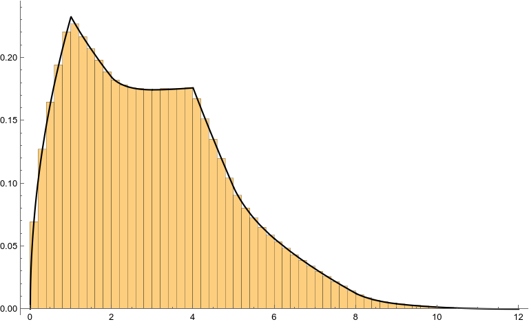
enter image description here

Footnote

  1. here $b-g\in\{0,1,4\}$ come from breaking the integrals up from $-1$ to $0$ and $0$ to $2$ so the new variables are $1$-to-$1$ with the old ones on those intervals.
$\endgroup$
7
  • 2
    $\begingroup$ +1. Thank you for your work. I need some time to think about it. $\endgroup$
    – user64494
    Commented Jul 29, 2021 at 19:33
  • $\begingroup$ Something to adjust: your formula is a histogram, not a formula. Next, if you mean $\delta(k)$ as the $\delta$-distribution, then the integral $$\int _{a-b}^{a-c}\int _{w-d}^{w-e}\int _{v-f}^{v-g}\frac{\delta (k) dkdvdw}{8 \sqrt{v-k} \sqrt{w-v} \sqrt{a-w}} $$ makes no sense in traditional math. $\endgroup$
    – user64494
    Commented Jul 30, 2021 at 5:02
  • $\begingroup$ I accept your workaround, though the important statements "The pieces will clearly have bounds that are integers" and "The general idea is the pieces will be at the values of $\sum_{i=1}^d a_i^2$ with $\sum_{i=1}^d a_i^2$ in dimension $d$" are not grounded. $\endgroup$
    – user64494
    Commented Jul 30, 2021 at 5:06
  • $\begingroup$ @user64494 what do you mean "your formula is a histogram"? My formula is the PDF, as requested. Why wouldn't that integral make sense? It seems perfectly fine to me, Mathematica can calculate it, and it's literally a recasting of the formula from Wikipedia. When you say my statements about the pieces are not grounded, you mean they're wrong or just not explained? $\endgroup$
    – bRost03
    Commented Jul 30, 2021 at 11:00
  • $\begingroup$ I mean a bad link. $\endgroup$
    – user64494
    Commented Jul 30, 2021 at 12:53
7
$\begingroup$

@bRost03 has the best answer. This following produces the desired function but not so neat and tidy. (Some parts of the result contains imaginary numbers although when evaluated result in a non-negative real number for the density. Maybe some simplification is possible.)

Because the density function is available for the 2D case, get the pdf's for the 1D and 2D case. In other words we're going to look for the pdf for

$$X_1^2+X_2^2+X_3^2 = (X_1^2+X_2^2)+X_3^2=Z_{12}+Z_3=Z$$

pdf12 = PDF[TransformedDistribution[x1^2 + x2^2, {x1 \[Distributed] UniformDistribution[{-1, 2}],
  x2 \[Distributed] UniformDistribution[{-1, 2}]}], z12]
pdf3 = PDF[TransformedDistribution[x^2, x \[Distributed] UniformDistribution[{-1, 2}]], z3]

To find the pdf for $Z$ multiply the two pdf's together and replace z3 with z-z12. This gives us the joint pdf for $Z$ and $Z_{12}$.

jointpdf = pdf12 pdf3 /. z3 -> z - z12 // PiecewiseExpand;

Note to (final?) update: I've removed the Do-loops and used the more standard Mathematica probability functions in what follows.

To find the pdf for $Z$ we obtain the marginal distribution of that bivariate pdf.

dist = ProbabilityDistribution[jointpdf, {z, 0, 12}, {z12, 0, 8}]
pdf = PDF[MarginalDistribution[dist, 1], z]

This result contains some imaginary numbers that cancel out when evaluated but those can be appropriately eliminated with the following:

pdf[[1, All, 1]] = FullSimplify[ComplexExpand[#[[1]], TargetFunctions -> {Re, Im}], 
  Assumptions -> #[[2]]] & /@ pdf[[1, All]];

Finally, we simplify the pdf:

pdf = pdf//Simplify

The result is

pdf = Piecewise[{{(-(1/27))*Pi*(-3 + Sqrt[z]), Inequality[1, Less, z, LessEqual, 2]}, {(2*Pi*Sqrt[z])/27, Inequality[0, Less, z, LessEqual, 1]}, {(1/54)*(-3*Pi + 12*ArcTan[2/Sqrt[-8 + z]] + 2*Sqrt[z]*(-ArcTan[Sqrt[z/(-8 + z)]] + ArcTan[(1/4)*Sqrt[(-8 + z)*z]])), Inequality[9, LessEqual, z, Less, 12]}, {(1/108)*(-5*Pi*(-3 + Sqrt[z]) + 12*ArcTan[2/Sqrt[-5 + z]] - 24*ArcTan[Sqrt[-5 + z]] + 2*Sqrt[z]*(2*ArcTan[2*Sqrt[(-5 + z)/z]] - 2*ArcTan[2*Sqrt[z/(-5 + z)]] - ArcTan[2/Sqrt[(-5 + z)*z]] + 2*ArcTan[(1/2)*Sqrt[(-5 + z)*z]] + ArcTan[(Sqrt[-5 + z]*z + 2*Sqrt[(-5 + z)*z])/(4 + 2*Sqrt[z])])), 6 < z < 8}, {(1/108)*(-9*Pi - 2*Pi*Sqrt[z] + 48*ArcTan[2/Sqrt[-8 + z]] + 12*ArcTan[2/Sqrt[-5 + z]] - 24*ArcTan[Sqrt[-5 + z]] + 2*Sqrt[z]*(ArcCot[2*Sqrt[z/(-5 + z)]] + 2*ArcTan[2*Sqrt[(-5 + z)/z]] - 4*ArcTan[Sqrt[z/(-8 + z)]] + 4*ArcTan[(1/4)*Sqrt[(-8 + z)*z]] - ArcTan[2/Sqrt[(-5 + z)*z]] - ArcTan[(2*z)/Sqrt[(-5 + z)*z]] + 2*ArcTan[(1/2)*Sqrt[(-5 + z)*z]] + ArcTan[(Sqrt[-5 + z]*z + 2*Sqrt[(-5 + z)*z])/(4 + 2*Sqrt[z])])), 8 < z < 9}, {(1/108)*(9*Pi - 4*ArcCot[2/Sqrt[3]] + 8*ArcTan[2/Sqrt[3]] - 2*Sqrt[2]*(3*Pi + ArcTan[(47940*Sqrt[6])/7199])), z == 8}, {(1/27)*(3*(Pi - 2*ArcTan[Sqrt[-2 + z]]) + Sqrt[z]*(ArcCsc[1 - z] + ArcTan[Sqrt[(-2 + z)/z]] - ArcTan[Sqrt[z/(-2 + z)]] + ArcTan[Sqrt[(-2 + z)*z]])), Inequality[2, Less, z, LessEqual, 3]}, {(1/54)*(5*Pi - ArcCot[2] + Sqrt[6]*ArcCot[2*Sqrt[6]] + 5*ArcTan[2] - Sqrt[6]*(5*ArcTan[Sqrt[2/3]] + 3*ArcTan[Sqrt[3/2]] + ArcTan[2*Sqrt[6]])), z == 6}, {(1/108)*(6*Pi + ArcTan[(45299420*Sqrt[2])/382087111]), z == 4}, {(1/108)*(9*Pi - 12*ArcTan[Sqrt[-2 + z]] + Sqrt[z]*(-2*ArcSec[1 - z] + 2*ArcTan[Sqrt[(-2 + z)/z]] - ArcTan[Sqrt[z/(-2 + z)]] + 2*ArcTan[Sqrt[(-2 + z)*z]] + ArcTan[2 - z - Sqrt[(-2 + z)*z], z + Sqrt[(-2 + z)*z]])), 3 < z < 4}, {(1/108)*(21*Pi - 8*Pi*Sqrt[z] + 24*ArcTan[2/Sqrt[-5 + z]] - 48*ArcTan[Sqrt[-5 + z]] - 12*ArcTan[Sqrt[-2 + z]] + 2*Sqrt[z]*(2*ArcCot[2*Sqrt[z/(-5 + z)]] + ArcCsc[1 - z] + 4*ArcTan[2*Sqrt[(-5 + z)/z]] + ArcTan[Sqrt[(-2 + z)/z]] - 2*ArcTan[2/Sqrt[(-5 + z)*z]] - 2*ArcTan[(2*z)/Sqrt[(-5 + z)*z]] + 4*ArcTan[(1/2)*Sqrt[(-5 + z)*z]] - ArcTan[Sqrt[z/(-2 + z)]] + ArcTan[Sqrt[(-2 + z)*z]] + 2*ArcTan[(Sqrt[-5 + z]*z + 2*Sqrt[(-5 + z)*z])/(4 + 2*Sqrt[z])])), 5 < z < 6}, {(1/108)*(Pi*(33 - 13*Sqrt[z]) - 12*ArcTan[Sqrt[-2 + z]] + Sqrt[z]*(2*ArcCsc[1 - z] + 2*ArcTan[Sqrt[(-2 + z)/z]] - ArcTan[Sqrt[z/(-2 + z)]] + 2*ArcTan[Sqrt[(-2 + z)*z]] + ArcTan[2 - z - Sqrt[(-2 + z)*z], z + Sqrt[(-2 + z)*z]])), 4 < z < 5}, {(1/216)*(58*Pi - 23*Sqrt[5]*Pi + 2*Sqrt[5]*ArcSin[7/128]), z == 5}}, 0]

Update: Below is all of the code in one place with approximate execution times:

(* About 12 seconds *)
pdf12 = PDF[TransformedDistribution[x1^2 + x2^2,
   {x1 \[Distributed] UniformDistribution[{-1, 2}],
    x2 \[Distributed] UniformDistribution[{-1, 2}]}], z12]
pdf3 = PDF[TransformedDistribution[x^2,
  x \[Distributed] UniformDistribution[{-1, 2}]], z3]
jointpdf = pdf12 pdf3 /. z3 -> z - z12 // PiecewiseExpand;
dist = ProbabilityDistribution[jointpdf, {z, 0, 12}, {z12, 0, 8}];

(* About 10 minutes *)
pdf = PDF[MarginalDistribution[dist, 1], z];

(* About 2 minutes *)
pdf[[1, All, 1]] = FullSimplify[ComplexExpand[#[[1]], TargetFunctions -> {Re, Im}],
     Assumptions -> #[[2]]] & /@ pdf[[1, All]];

(* About 1 second *)
pdf = pdf // Simplify
$\endgroup$
18
  • $\begingroup$ Thank you. Some places which I don't understand: "Now find the joint pdf for $Z$ and $Z−X_{12}$" and "Integrate out $Z_{12}$ "($Z_{12}$ is a random variable.). Could you explain those? There are other unclear pieces too. TIA. $\endgroup$
    – user64494
    Commented Jul 31, 2021 at 19:05
  • $\begingroup$ $X_{12}$ should have been $Z_{12}$. And I've modified the notion a bit so hopefully things are more standard. $\endgroup$
    – JimB
    Commented Jul 31, 2021 at 21:10
  • $\begingroup$ Sorry, still don't understand " integrate out z12:". $\endgroup$
    – user64494
    Commented Aug 1, 2021 at 4:37
  • $\begingroup$ The quick answer is at en.wikipedia.org/wiki/Convolution_of_probability_distributions. I'll add more details tomorrow. $\endgroup$
    – JimB
    Commented Aug 1, 2021 at 5:30
  • $\begingroup$ +1.Thank you. I got it. Poor comments make it difficult to understand a good job. $\endgroup$
    – user64494
    Commented Aug 1, 2021 at 13:49

Your Answer

By clicking “Post Your Answer”, you agree to our terms of service and acknowledge you have read our privacy policy.

Not the answer you're looking for? Browse other questions tagged or ask your own question.