How to add an attractive potential (migration term) named component to Mass Transport PDE

Question

Wolfram Mathematica 12.2 now features "Named Partial Differential Equation Terms"

For specific physics fields, relevant PDE terms have been packaged as components and augmented with boundary condition functions typically encountered in the field.

I'm interested in Mass Transport PDEs and Boundary Conditions and particularly on how to introduce a migration term, i.e a physical potential or force terms to a diffusion problem. This is to model the time evolution of the probability to find diffusing particles experiencing forces in solution.

An example PDE without potentials is

With[
 {
  length = 500,
  height = 30
  },
 Ω = Rectangle[{0, 0}, {length, height}]; (* Domain *)
 pars = <| (* Parameters *)
   "DiffusionCoefficient" -> 10,
   Vavg -> 10,
   "MassConvectionVelocity" -> {2 Vavg*(1 - ((y - height/2)/(height/2))^2), 0},
   "Method" -> "StiffnessSwitching"
   |>;
 vars = {c[t, x, y], t, {x, y}}; (* Variables *)
 Gin = MassConcentrationCondition[x == 0, vars, pars, <|"MassConcentration" -> 0|>];
 Gbottom = 
  MassFluxValue[
  y == 0,
  vars, 
  pars,
  <|"MassFlux" -> 2 UnitBox[(x - 100)/50] Exp[-(1/2) (t - 2)^2], 
    "BoundaryUnitNormal" -> {0, 1}|>];
 Gtop = MassImpermeableBoundaryValue[y == height, vars, pars, <|"BoundaryUnitNormal" -> {0, -1}|>];
 ics = { c[0, x, y] == 0};
 pde = {
   MassTransportPDEComponent[vars, pars] == Gtop + Gbottom
   , Gin
   , ics
   };
 ]

With solution

First@AbsoluteTiming[
  cfun = NDSolveValue[
     pde
     , c
     , {t, 0, 20}
     , {x, y} ∈ Ω
     , InterpolationOrder -> 2
     , AccuracyGoal -> 14
     , Method -> Automatic
     , MaxStepFraction -> 1/6000
     ];
  ]

How do I add an attractive potential using the packaged named terms?

For the interested reader, think Smoluchowski or Fokker-Planck equations as described in chapter 4 here.

Answer 1

I am anything else than an expert in statistics and I can not directly answer your question. However, I can show how I modeled a Fokker-Planck equation in the hope that this helps you move forward. I Have grabbed the first PDF that a search for FEM + Fokker-Planck gave me and I am going to show how to replicate that example.

Before I do that, I'd like to point you to an undocumented function that shows the string parameter names a specific PDE component responds to:

PDEModels`PDEModelParameters[MassTransportPDEComponent]

{"DiffusionCoefficient", "MassConvectionVelocity", \
"MassReactionRate", "MassSource", "ModelForm"}

Next, I'd like to model equation 7 from the mentioned paper, which is a Fokker-Planck equation. To do so, I myself go in steps. I start with a default setup.

vars = {c[t, x, y], t, {x, y}};
pars = <||>;
MassTransportPDEComponent[vars, pars]

Inactive[Div][{{-1, 0}, {0, -1}} . Inactive[Grad][c[t, x, y], {x, y}], 
  {x, y}] + Derivative[1, 0, 0][c][t, x, y]

First, I set the diffusion coefficient such that it corresponds to the one one in the paper. This is symbolic for now.

pars["DiffusionCoefficient"] = {{0, 0}, {0, D}};
MassTransportPDEComponent[vars, pars]

Inactive[Div][{{0, 0}, {0, -D}} . Inactive[Grad][c[t, x, y], {x, y}], 
  {x, y}] + Derivative[1, 0, 0][c][t, x, y]

Next is the conservative convection part. Conservative vs. non-conservative is explained in the ref page or in the MassTransport tutorial

pars["ModelForm"] = "Conservative";
pars["MassConvectionVelocity"] = {y, -2 \[Xi] \[Omega] y - x};
MassTransportPDEComponent[vars, pars]

Inactive[Div][{{0, 0}, {0, -D}} . Inactive[Grad][c[t, x, y], {x, y}], 
  {x, y}] + Inactive[Div][{y*c[t, x, y], (-x - 2*y*\[Xi]*\[Omega])*c[t, x, y]}, 
  {x, y}] + Derivative[1, 0, 0][c][t, x, y]

To cross check this I used:

temp = MassTransportPDEComponent[{p[t, x, y], {x, y}}, pars];
(-temp) // Activate // Simplify

This should be equivalent to equation 8 from the paper.

Now, we set up the parameters.

rules = {\[Mu] -> {5, 5}, \[Sigma] -> 1/9*IdentityMatrix[2], \[Xi] -> 
   1/20, \[Omega] -> 1, D -> 1/10}

We could very well also put these in pars.

The initial condition:

ics = c[0, x, y] == 
  PDF[MultinormalDistribution[\[Mu], \[Sigma]] /. rules, {x, y}]

The boundary condition:

G1 = NeumannValue[0, True]

(we do not really need this)

Domain and time:

\[CapitalOmega] = Rectangle[{-10, -10}, {10, 10}];
tEnd = 100;

According to the paper, a first order mesh is OK:

Needs["NDSolve`FEM`"]
mesh = ToElementMesh[\[CapitalOmega], MaxCellMeasure -> 0.05, 
   "MeshOrder" -> 1];
mesh["Wireframe"]

Now we solve the equation, note that this can be memory consuming, also mentioned in the paper.

op = MassTransportPDEComponent[vars, pars];
if = Monitor[
  NDSolveValue[{op == G1, ics} /. rules, 
   c, {t, 0, tEnd}, {x, y} \[Element] mesh, 
   EvaluationMonitor :> (monitor = Row[{"t = ", CForm[t]}])], monitor]

Visualize:

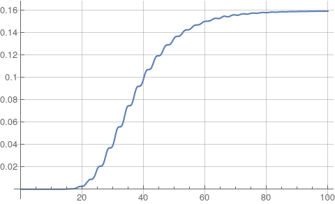
Plot[if[t, 0, 0], {t, 0, tEnd}, 
 Ticks -> {Automatic, Range[0, 0.18, 0.02]}, 
 GridLines -> {Automatic, Range[0, 0.18, 0.02]}]

which replicates figure 1 from the paper.

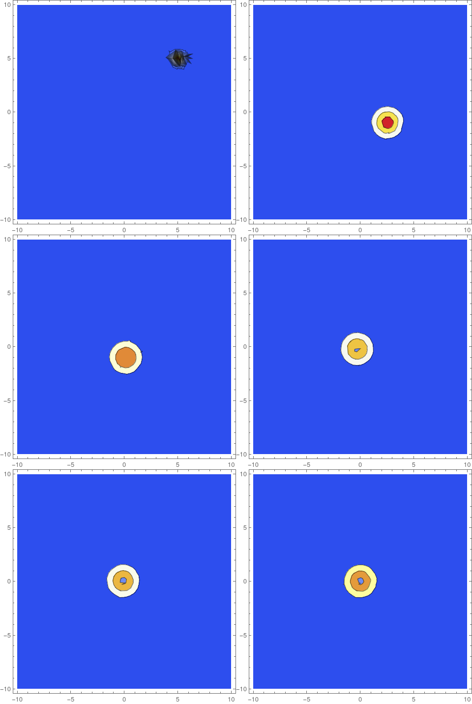
frames = ContourPlot[if[#, x, y], {x, y} \[Element] \[CapitalOmega], 
     PlotRange -> All, ColorFunction -> "TemperatureMap", 
     Contours -> Range[0.05, 2, 0.05]] & /@ Range[0, tEnd, 1];

ListAnimate[frames]

Update

The explicit example you requested can be done along the same procedure from above.

vars = {p[t, x], t, {x}};
pars = <||>;
pars["DiffusionCoefficient"] = {{D}};
pars["ModelForm"] = "Conservative";
(* Eqn 4.17 ff *)
potential[x_] := c x
pars["MassConvectionVelocity"] = \[Beta] *(-Grad[potential[x], {x}]);
MassTransportPDEComponent[vars, pars]

Inactive[Div][{{-D}} . Inactive[Grad][p[t, x], {x}], {x}] + 
 Inactive[Div][{-(c*\[Beta]*p[t, x])}, {x}] + Derivative[1, 0][p][t, x]

Set up some parameters, the region and the analytical solution:

\[CapitalOmega] = Line[{{-s}, {s}}] /. s -> 8;
rules = {D -> 1, \[Beta] -> 1, c -> 1};
anaSol[t_, x_] := Evaluate[With[{x0 = 0, t0 = 0},
    1/Sqrt[4 \[Pi] D (t - t0)]*
     Exp[-(x - x0 + D \[Beta] c (t - t0))^2 / (4 D *(t - t0))]] /. 
   rules]

Generate the initial conditions:

tStart = 1/10;
ics = p[tStart, x] == anaSol[tStart, x];

Solve the PDE:

op = MassTransportPDEComponent[vars, pars] /. rules;
tEnd = 1;
if = NDSolveValue[{op == 0, ics}, 
  p, {t, tStart, tEnd}, {x} \[Element] \[CapitalOmega]]

Visualize:

Manipulate[
 Plot[{anaSol[t, x], if[t, x]}, {x} \[Element] \[CapitalOmega], 
  PlotRange -> All], {t, tStart, tEnd}]

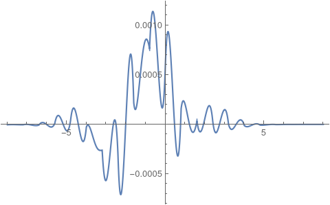
Error:

Plot[{anaSol[tEnd, x] - if[tEnd, x]}, {x} \[Element] \[CapitalOmega], 
 PlotRange -> All]

Answer 2

From my reading of the documentation for the MassTransportPDEComponent, it appears to be currently missing the ability to add a migration term. Consider, for example, the Nernst-Planck equation:

$$\frac{{\partial {c_i}}}{{\partial t}} + \nabla \cdot\underbrace {\left( { - {D_{AB}}\nabla {c_i} - {c_i}{\bf{u}} + {z_i}{u_i}{c_i}E} \right)}_{{{\bf{N}}_i}} - {R_i} = 0$$

Where

$${{\bf{N}}_i} = - \overbrace {{D_i}\nabla {c_i}}^{Diff} - \overbrace {{c_i}{\bf{u}}}^{Conv} + \overbrace {{z_i}{u_i}{c_i}E}^{Migr}$$

It is not difficult to add a migration term through the use of the PDE building block DerivativePDETerm. In coefficient form, the PDE may be expressed as:

$$m\frac{{{\partial ^2}}}{{\partial {t^2}}}u + d\frac{\partial }{{\partial t}}u + \nabla \cdot\left( { - c\nabla u - \alpha u + \gamma } \right) + \beta \cdot\nabla u + au - f = 0$$

Therefore, $\gamma=Migration=DerivativePDETerm$. Here is an example how we can add it to the pde:

With[{length = 500, height = 30}, Ω = 
  Rectangle[{0, 0}, {length, height}];(*Domain*)
 pars = <|(*Parameters*)"DiffusionCoefficient" -> 10, Vavg -> 10, 
   "MassConvectionVelocity" -> {2 Vavg*(1 - ((y - height/2)/(height/
             2))^2), 0}, "Method" -> "StiffnessSwitching"|>;
 vars = {c[t, x, y], t, {x, y}};(*Variables*)
 Gin = MassConcentrationCondition[x == 0, vars, 
   pars, <|"MassConcentration" -> 0|>];
 Gbottom = 
  MassFluxValue[y == 0, vars, 
   pars, <|"MassFlux" -> 
     2 UnitBox[(x - 100)/50] Exp[-(1/2) (t - 2)^2], 
    "BoundaryUnitNormal" -> {0, 1}|>];
 Gtop = MassImpermeableBoundaryValue[y == height, vars, 
   pars, <|"BoundaryUnitNormal" -> {0, -1}|>];
 ics = {c[0, x, y] == 0};
 pde = {MassTransportPDEComponent[vars, pars] + 
     DerivativePDETerm[vars, {- 8 c[t, x, y], c[t, x, y]}] == 
    Gtop + Gbottom, Gin, ics};]

Now, we can set up and solve the system and observe that it is different from the original solution.

First@AbsoluteTiming[
  cfun = NDSolveValue[pde, 
     c, {t, 0, 20}, {x, y} ∈ Ω, 
     InterpolationOrder -> 2, AccuracyGoal -> 14, Method -> Automatic,
      MaxStepFraction -> 1/6000];]
DensityPlot[cfun[20, x, y], {x, y} ∈ Ω, 
 ColorFunction -> "SunsetColors", AspectRatio -> Automatic, 
 ImageSize -> 800]

Original solution:

There could be implications for how this term interacts with boundary conditions. You may want to request a migration term be added to the MassTransportPDEComponent to the Future enhancements for the finite element method page to ensure that it gets handled properly.