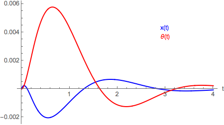
In this documentation article, Regulate an Inverted Pendulum, the author started by creating the following system.
pendulum =
  StateSpaceModel[
    {(M + m) x''[t] - m l Sin[θ[t]] θ'[t]^2 + m l Cos[θ[t]] θ''[t] ==
       F[t] + d[t] Cos[θ[t]],
     m x''[t] Cos[θ[t]] + m l θ''[t] == m g Sin[θ[t]] + d[t]},
    {θ[t], θ'[t], x[t], x'[t]},
    {F[t], d[t]},
    {θ[t], x[t]},
    t] /. {M -> 5.6, m -> 0.53, l -> 0.85, g -> 9.8};

poles = {-1 + 2 I, -1 - 2 I, -5, -7};
Then he got the feedback gains
k =
  Join[
    StateFeedbackGains[SystemsModelExtract[pendulum, 1], poles],
    ConstantArray[0, 4]}]
and plotted the output response with x and θ, keeping θ close to zero, with the following
Plot[
  OutputResponse[
    SystemsModelStateFeedbackConnect[pendulum, k],
    {0,UnitStep[t] - UnitStep[t - 1]},
    {t, 4}] // Evaluate,
  {t, 0, 4},
  PlotRange -> All,
  PlotStyle -> {Blue, Red},
  Epilog ->
    Inset[Column[{Style["x(t)", 10, Blue], Style["θ(t)", 10, Red]}], {3, 0.004}],
  AxesLabel -> {"t"}]
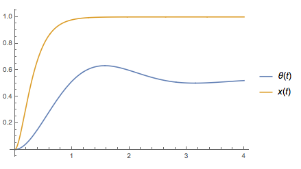
My question is how to pass the desired position and angle he wants the system to stabilize at; i.e., x = 1, θ = π/6


d[t]applied at right angles to the pendulum. Expectd[t]to swing negative when $\theta$ is positive. Also, the system model has outputs $\{\theta [t], x[t]\}$ in that order, so the blue curve is $\theta$ and the red one is $x$, if I'm not mistaken. $\endgroup$