47
$\begingroup$

Today I was playing with Peter de Jong attractor.

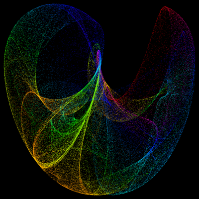
At the bottom of the page I've linked there are beautiful examples like: enter image description here
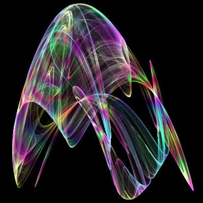
My attempts are not so great:

enter image description here

It is around 10^5 points. For more than 5*10^5 my 4GB RAM gives up. How can I achieve such smooth result on standard/oldish pc?


Here is the piece of code to play with:

Points generator:

fr2 = Compile[{{p, _Real, 1}, {n, _Integer}, {a, _Real, 1}, {b, _Real, 1},
               {c, _Real, 1}},
   NestList[
    { Sin[a[[1]] #[[2]]] - Cos[a[[2]] #[[1]]],
      Sin[b[[1]] #[[1]]] - Cos[b[[2]] #[[2]]],
      Sin[c[[1]] #[[1]]] - Cos[c[[2]] #[[1]]]
      } &, p, n]];

Interactive toy:

For printed color image I've used approach introduced by Szabolcs in antialiasing3D.

DynamicModule[{a, b, c, n, type, fig, controls, print},
 Deploy@Dynamic[Refresh[
    Panel@Grid[{{fig, controls}}, Spacings -> 2],
    None]],

 Initialization :> (
   type = 1;
   n = 100000;
   {a, b, c} = {{1.4, -2.3}, {2.4, -2.1}, {2.41, 1.64}};

   controls = Column[{
      Slider2D[Dynamic@a, {-Pi, Pi, .01}], Dynamic@a,
      Slider2D[Dynamic@b, {-Pi, Pi, .01}], Dynamic@b,
      Slider2D[Dynamic@c, {-Pi, Pi, .01}], Dynamic@c,
      Button["Print", print[], Method -> "Queued"] }];

   fig = Graphics[{White, AbsolutePointSize@1, 
      Dynamic[
       Point@fr2[{.0, .0, .0}, ControlActive[2 10^4, 10^5], a, b, c][[All , ;; 2]]]
      }, ImageSize -> {1, 1} 500, Background -> Black, AspectRatio -> Automatic];

   print[] := With[{t = 3, pointsize = 1, pts = 10^5, res = 72},
     Composition[
       CreateDocument,
       ImageResize[Rasterize[#, "Image", ImageResolution -> t res], Scaled[1/t]] &,
       Graphics[{AbsolutePointSize@pointsize, 
          Riffle[Hue@Rescale[#, {-2, 2}, {0, 1}] & /@ #[[;; , 3]], 
             Point /@ #[[;; , ;; 2]]] &@#
          }, ImageSize -> 800, Background -> Black] &
       ][fr2[{.0, .0, .0}, pts, a, b, c]]];
   )]
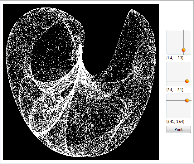
enter image description here

$\endgroup$
6
  • 3
    $\begingroup$ Just related, here is a demonstration project from @vitaliy-kaurov $\endgroup$
    – Murta
    Commented Jun 15, 2014 at 14:12
  • 4
    $\begingroup$ The first image you showed is made with 12 million points. They do not keep all the points in memory; whenever each point is computed they just set the corresponding pixel location in the image and move on. This way they don't need gigabytes of storage. $\endgroup$
    – user484
    Commented Jun 15, 2014 at 14:19
  • $\begingroup$ Google "Flame fractals". I create this type of fractals a lot; 10⁵ is not nearly enough iterations. You would like about 2000 iterations PER PIXEL in the final image to get a decent result. $\endgroup$ Commented Jun 16, 2014 at 6:55
  • $\begingroup$ @Paxinum Well, I understand :) Wanna share with us some fancy code/results? :) $\endgroup$
    – Kuba
    Commented Jun 16, 2014 at 7:15
  • 3
    $\begingroup$ @Kuba: The implementation I have is written in Java, and is open-sourced here: sourceforge.net/projects/flamethyst Some images created can be found here: people.su.se/~peal0658/index.php?page=fractals $\endgroup$ Commented Jun 16, 2014 at 8:02

3 Answers 3

40
$\begingroup$

UPDATE I thought it would be neat to try and animate the thing, so I let the $a$ parameter run between $-\pi$ and $\pi$. I generated 600 images and put them together using ffmpeg. Check it out on youtube.

It might not be in the spirit of Mathematica Stack Exchange, but allow me an objection - stuff that is slow in Mathematica should be kept out of it. To wit consider how this little C++ nugget does the grunt work:

#include <stdio.h>
#include <cmath>
#include <omp.h>

int main()
{
    const int dim = 4096;
    const float a = 1.4f, b = -2.3f, c = 2.4f, d = -2.1f;

    int size = dim*dim;
    float *image = new float[size];
    for (int i = 0; i < size; ++i) image[i] = 1;

    #pragma omp parallel
    {
        float x = omp_get_thread_num(), y = 0;
        for (int i = 0; i < 10000000; ++i)
        {
            float xn = sin(a * y) - cos(b * x);
            y = sin(c * x) - cos(d * y);
            x = xn;

            auto xp = ((dim - 1) * (1 + x * 0.43) * 0.5);
            auto yp = (int)((dim - 1) * (1 - y * 0.43) * 0.5);
            image[(int)((yp * dim + xp))] *= 0.99f;
        }
    }

    FILE *file = fopen("image.bin", "wb");
    fwrite(image, sizeof(float), size, file);
    fclose(file);
    delete[] image;
    return 0;
}

This should be compiled with fast math for better performance. I've also included omp in there, because my system has 12 cores and if I don't use them for this - there's no justification for me buying it.

And this Mathematica code makes an image and colorizes it from the produced data:

buffer = BinaryReadList["image.bin", "Real32"];
dim = Sqrt[Length@buffer];
bigimg = Image[Partition[buffer, dim], "Real32"];
Colorize[Rasterize[bigimg, ImageSize -> dim/4], 
ColorFunction -> ColorData["SunsetColors"]]

Note that I'm rendering the original on the 4096x4096 canvas, and then down-sampling it in Mathematica - which I find produces a more pleasant aesthetic. This stuff would have taken several days to do proper in C++, and while I'm sure it's possible to write a fast iterator in Mathematica - it would probably take a long time as well.

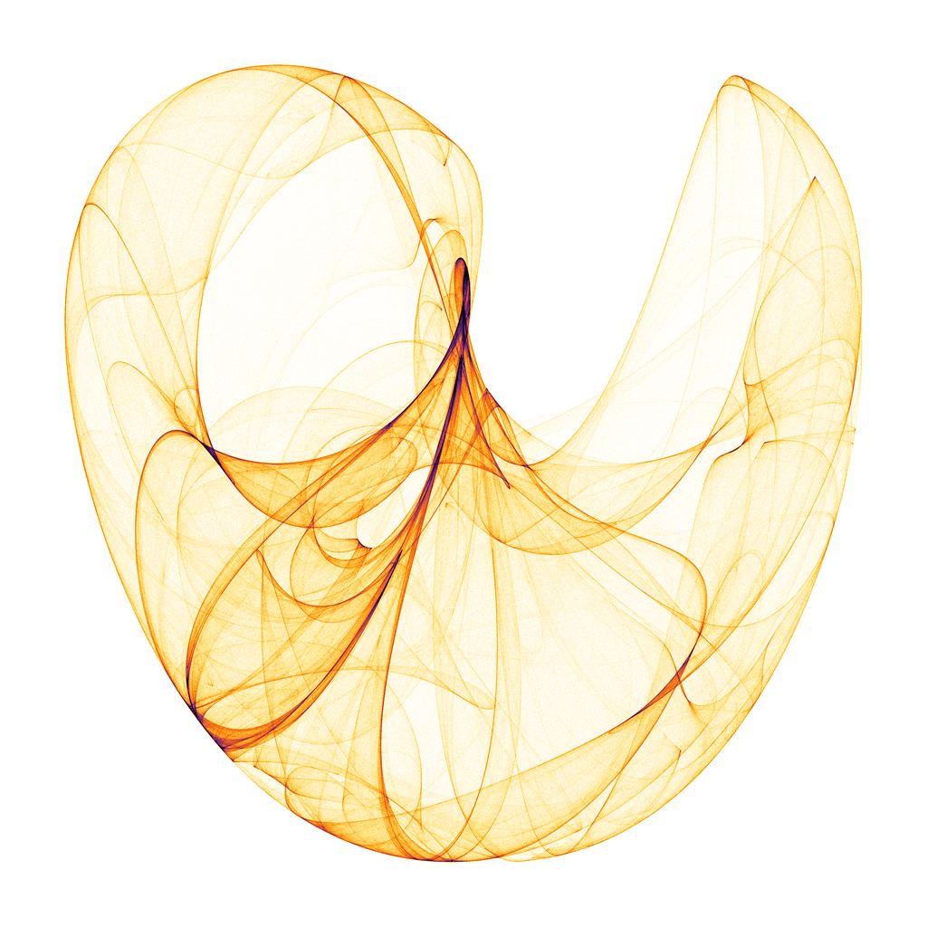
Final image:Thingy

$\endgroup$
6
  • 6
    $\begingroup$ Nice! BTW, this approach (using Java/C/C++ with Mathematica) is quite common on this site and even encouraged when appropriate (as it is in this case). Welcome to the site (even though you've had an account for ~2 years) :) $\endgroup$
    – rm -rf
    Commented Jun 17, 2014 at 17:24
  • 1
    $\begingroup$ @rm-rf Thanks. I used to be quite a Mathematica buff back in the day when there was no separate site. ;) $\endgroup$
    – Gleno
    Commented Jun 17, 2014 at 17:38
  • 1
    $\begingroup$ Öska, that error message means that you are not running the latest compiler; try adding -std=c++0x compilation flag. Then, since I was greedy and added openmp, you should add -fopenmp flag as well (assuming GCC). I compiled and ran this on windows under latest visual studio. $\endgroup$
    – Gleno
    Commented Jun 17, 2014 at 19:46
  • $\begingroup$ That's great you've decided to post that answer :) $\endgroup$
    – Kuba
    Commented Jun 17, 2014 at 20:02
  • 3
    $\begingroup$ @Gleno Works like a charm with g++ -std=c++0x -fopenmp file.cpp indeed, thanks. $\endgroup$
    – Öskå
    Commented Jun 18, 2014 at 9:21
37
$\begingroup$

As @RahulNarain says, forming the image point by point saves significant memory because the number of image pixels is typically much smaller than the hundreds of millions of iterations that compose it. Therefore, iterate the attractor equations, and for each point generated, find its location within the image matrix. Colour coding of the number of hits in each pixel makes the image.

The following is a rough example.

{a, b, c} = {{1.4, -2.3}, {2.4, -2.1}, {2.41, 1.64}};
Block[{xmin=-2., xmax=2., ymin=-2., ymax=2., delta=0.01, bins, d,
       itmax=10^5, x, y, tx, ty},
   bins = ConstantArray[0, Floor[{xmax-xmin, ymax-ymin}/delta] + {1, 1}];
   d = Dimensions[bins];
   {x, y} = {0., 0.};
   Do[
      {x, y} = {Sin[a[[1]] y] - Cos[a[[2]] x], 
                Sin[b[[1]] x] - Cos[b[[2]] y]};
      tx = Floor[(x - xmin)/delta] + 1;
      ty = Floor[(y - ymin)/delta] + 1;
      If[tx >= 1 && tx <= d[[1]] && ty >= 1 && ty <= d[[2]], 
         bins[[tx, ty]] += 1],
      {i, 1, itmax}];
   ArrayPlot[Log[bins+1], ColorFunction->(ColorData["DarkRainbow",#^0.4]&)]]

This block may be compiled in the usual way. Other plotting routines such as MatrixPlot or ListDensityPlot may be used. TheLog[bins+1]function and the exponent within theColorFunctionare example methods to adjust the dynamic range of pixel counts to bring out subtle features.

COMPILED CODE

attractor =
   Compile[{{xmin,_Real}, {xmax,_Real}, {ymin,_Real}, {ymax,_Real},
            {delta,_Real}, {itmax,_Integer}, {a,_Real,1}, {b,_Real,1}},
   Block[{bins, d, x, y, tx, ty},
      bins = ConstantArray[0, Floor[{xmax-xmin, ymax-ymin}/delta] + {1,1}];
      d = Dimensions[bins];
      {x, y} = {0., 0.};
      Do[
         {x, y} = {Sin[a[[1]] y] - Cos[a[[2]] x], 
                   Sin[b[[1]] x] - Cos[b[[2]] y]};
         tx = Floor[(x - xmin)/delta] + 1;
         ty = Floor[(y - ymin)/delta] + 1;
         If[tx >= 1 && tx <= d[[1]] && ty >= 1 && ty <= d[[2]], 
            bins[[tx, ty]] += 1],
         {i, 1, itmax}];
      bins],
      CompilationTarget :> "C"];

Example run:

AbsoluteTiming[bins = N[attractor[-2., 2., -2.2, 2.2, 0.005, 5*10^6,
                                  {1.2, -2.1}, {2.4, -2.1}]];]
ArrayPlot[Log[bins+1], ColorFunction->(ColorData["FallColors",#^0.4] &)]

EDIT

Thanks @Kuba for your many questions and answers on this site.

I compiled the above code for speed. I also wrote a Mathematica interface to Fortran code which allows me to rapidly calculate hundreds of millions of iterations. That way aManipulatecan quickly find the parameters giving an interesting form. The resulting matrix of number of hits in each pixel may be converted to an image via the built-in colour functions, opacity, etc.

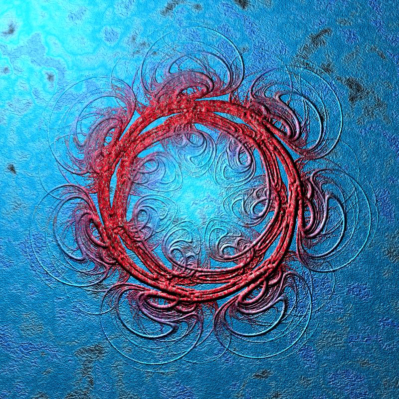
This image is formed with random affine transforms in the hyperbolic plane.

AffineHyperbolic

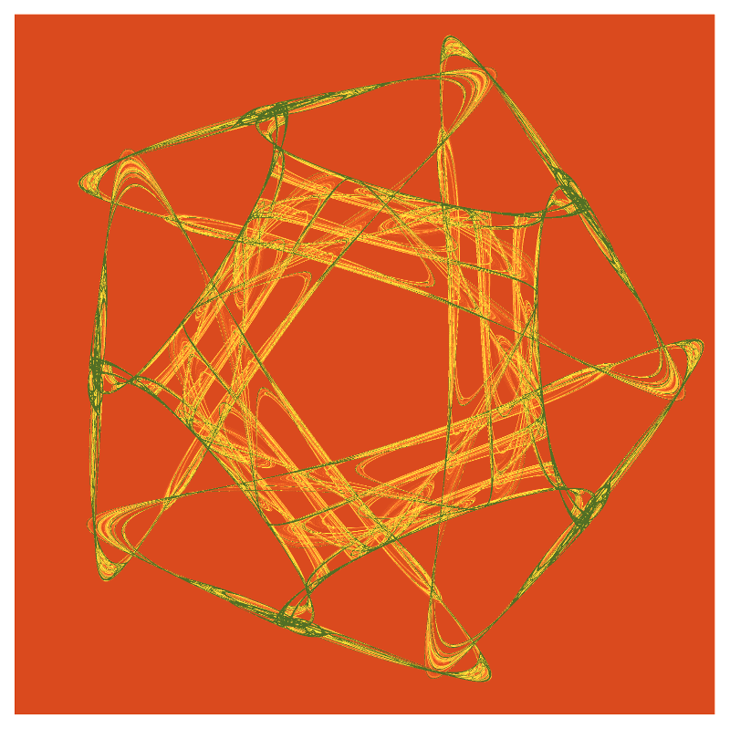
The following is a very simple 5-fold icon from the Symmetry In Chaos reference. FiveFoldSymChaos

But the really interesting (for me) images are made by converting the number of hits in each pixel to spheres with radii (non-linearly) proportional to the number of hits. The POVRay ray tracer (or other similar tool) "blobs" these spheres together, then textures may be applied. I have not as much experience with the Mathematica textures.

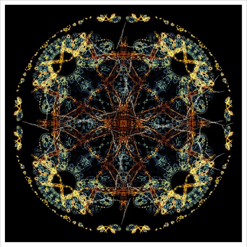
My Stack Exchange icon is derived from the Symmetry In Chaos equation, then inverted in its bounding circle to have matching inner and outer loops.

SevenLoopsInverted

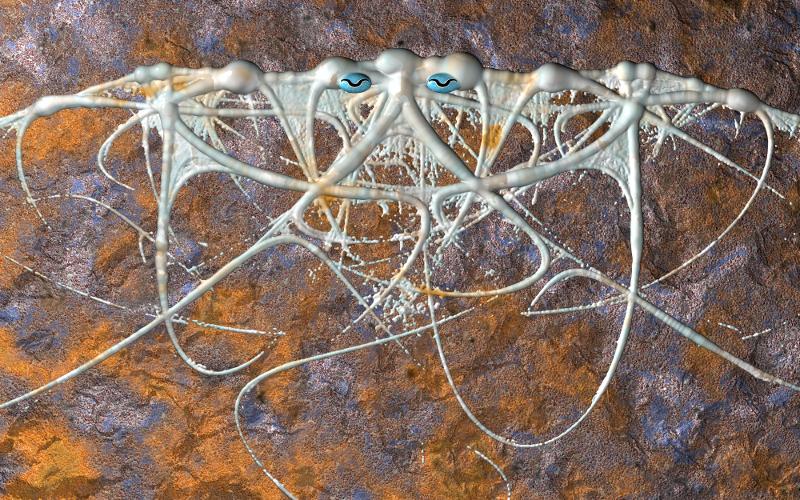
Other manipulations include a Moebius transform to open up the generally circular symmetry into a half plane. Cuttle fish eyes added for effect...

CuttleFish

$\endgroup$
7
  • 4
    $\begingroup$ Nice! i.sstatic.net/YxIgU.png $\endgroup$
    – rm -rf
    Commented Jun 15, 2014 at 21:17
  • 3
    $\begingroup$ Here's an animation where $a_1 \in [-2,2]$. $\endgroup$
    – wxffles
    Commented Jun 16, 2014 at 0:55
  • 5
    $\begingroup$ @KennyColnago Great reference, thanks :) p.s. don't you know that without pictures posts get half the upvotes they can? :p $\endgroup$
    – Kuba
    Commented Jun 16, 2014 at 6:00
  • 2
    $\begingroup$ I think it'll be better if you add the compiled code since the existed piece of code can't be compiled directly. Compile isn't easy for everyone :) $\endgroup$
    – xzczd
    Commented Jun 18, 2014 at 7:46
  • 2
    $\begingroup$ compiled code example has been included $\endgroup$ Commented Jun 19, 2014 at 15:09
26
$\begingroup$

I revisited this problem - this time in pure Mathematica. The trick to any kind of performance is the Compile[] function, which in itself can be a bit moody - so you need to set global options to warn you when it refuses compilation and work around that. The performance I'm seeing is on the order of magnitude slower than that I get from C++, and two orders of magnitude slower than I get with C++ AMP (GPGPU on Windows; I used AMP to generate images for this animation).

Another point of note, is that I've discovered that the algorithm starting points actually matter! If you take a uniform sample in the region $[-2, 2]$ as starting points, instead of $(x_0, y_0) = (0, 0)$ you get a slightly different image, typically with more artifacts. As I've tried to animate the $a$ parameter of the equations going from $-\pi$ to $\pi$, starting with $(x_0, y_0) = (0, 0)$ produces random blank frames for some values of $a$, while selecting points uniformly produces a smooth animation.

Anyway, the Mathematica code for the $(x_0, y_0) = (0, 0)$ case is as follows:

func = Compile[{{dim, _Integer}, {params, _Real, 
     1}, {iters, _Integer}},
   Module[{matrix, d1, d2, a, b, c, d, x, y, iter, xp, xn, yp, yn, 
     max},
    matrix = Table[0.0, {dim dim}];
    {a, b, c, d, x, y, iter} = params~Join~{0, 0, 1};
    {d1, d2} = {1 + 0.5 (dim - 1), 0.25 (dim - 1)};
    While[++iter < iters,
     xn = Sin[a y] - Cos[b x]; y = Sin[c x] - Cos[d y]; x = xn;
     xp = Floor[d1 + d2 x]; yp = Floor[d1 - d2 y];
     ++matrix[[yp dim + xp]];
     ];
    max = Max@matrix;
    Partition[(Sqrt[#]/max &) /@ matrix, dim]
    ], CompilationTarget -> "C", RuntimeOptions -> "Speed"];

dejong[dim_, params_, iters_] := Module[{matrix},
   matrix = func[dim, params, iters];
   Colorize[ArrayPlot[matrix, ImageSize -> dim, Frame -> False],
    ColorFunction -> ColorData["SunsetColors"]]];

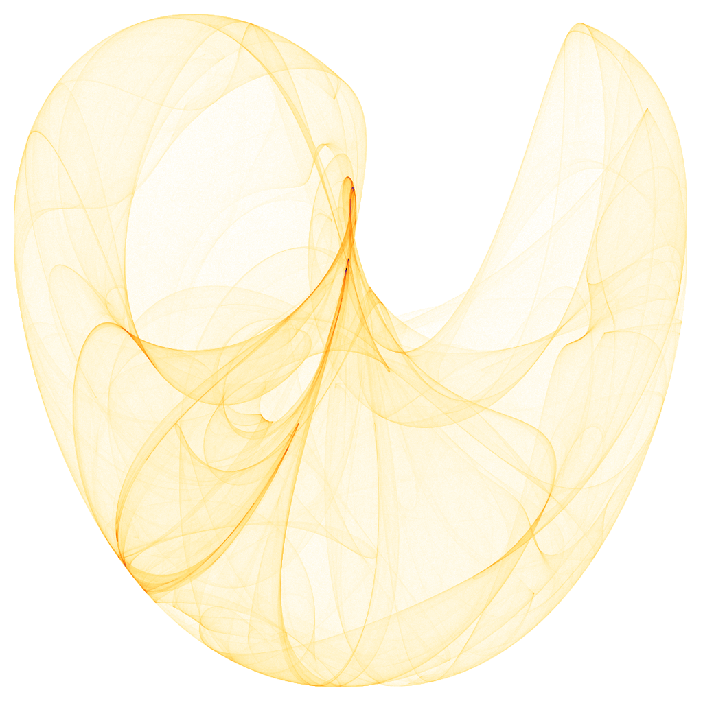
You can get a value matrix by calling func, or an image by calling dejong. Example would be:

dejong[1024, {1.4, -2.3, 2.4, -2.1}, 20000000]

Which in roughly 2 seconds produces:

Output Image

Faster output can be generated in black and white, if you forgo the colorization step, which takes roughly half the time.

$\endgroup$
2
  • $\begingroup$ Nice to mention the artifacts, I've enconutered them as well when I wrote my code to generate such images and was surprised when I couldn't see them in other images. $\endgroup$
    – shrx
    Commented Jul 6, 2014 at 21:06
  • 5
    $\begingroup$ I'd like to mention that, the "CompileOptions" set in $CCompiler will significantly influence the speed of the code in this case. For GCC, Mathematica uses "CompileOptions"->"-O2" by default, but when I changed it to "CompileOptions"->"-Ofast", I got a 2X speed-up! BTW, with my dual core old machine, your C++ code is even a little slower than the Mathematica code with -Ofast. $\endgroup$
    – xzczd
    Commented Oct 15, 2014 at 10:08

Your Answer

By clicking “Post Your Answer”, you agree to our terms of service and acknowledge you have read our privacy policy.

Not the answer you're looking for? Browse other questions tagged or ask your own question.