Schrödinger eigenvalue problem in two dimensions (Harmonic Oscillator)

Question

I read here the discussion about how to solve a one-dimensional eigenvalue problem. I am wondering, how can one generalize these methods to two dimensions?

For example, how to solve this equation:

$$-(d^2/dx^2+d^2/dy^2)u(x,y)+(x^2+y^2+xy)u(x,y)=Eu(x,y)$$

or any other potentials?

What about three dimensions? Is there any general procedure?

Answer 1

In order to give one possible answer, I'll just take the isotropic harmonic oscillator in 2D and do a finite-difference calculation by discretizing the xy plane with constant spacing a.

Here is the construction of the resulting matrix for the Hamiltonian, h. I assume the origin of our spatial grid (where the potential minimum is) lies at {0,0}, and the number of grid points in all directions from the origin is nX. Each grid step corresponds to a length of a = 0.2. On this grid, I then define the potential energy as a function v[x_, y_], and evaluate it at the grid points to create the 2D matrix vGrid. But this is the easy part.

Now we have to make a matrix out of the Hamiltonian in the space of tuples of {x,y} positions. This means the rows and columns of the matrix that we want to diagonalize are labeled by the entries of a list of tuples, which I call xyList. The Hamiltonian has one term that corresponds to the potential energy, and it is created in the above basis of tuples by taking the entries of the matrix vGrid corresponding to the tuple labeling each diagonal element of the Hamiltonian. This happens in the DiagonalMatrix term.

Finally, we have to construct the kinetic energy, i.e., the Laplacian. This is the only off-diagonal part of the matrix. How far off the diagonal its matrix elements extend depends on the order of the finite-difference approximation by which we replace the second derivatives in the Laplacian. Here I chose the simplest possible approximation.

nX = 20;
a = .2;

Clear[v];
v[x_, y_] := 1/2 (x^2 + y^2)

vGrid = Table[v[a i, a j], {i, -nX, nX}, {j, -nX, nX}];

xyList = Tuples[Range[1, 2 nX + 1], 2];

Timing[
 h = DiagonalMatrix[
     SparseArray[(vGrid[[##]] & @@@ xyList) + 2/a^2]] - 
    1/(2 a^2) AdjacencyMatrix[GridGraph[{2 nX + 1, 2 nX + 1}]];]

(* ==> {0.009491, Null} *)

v = Eigenvectors[h, -10];

ListDensityPlot[Partition[v[[10]], 2 nX + 1], 
 PlotRange -> All]

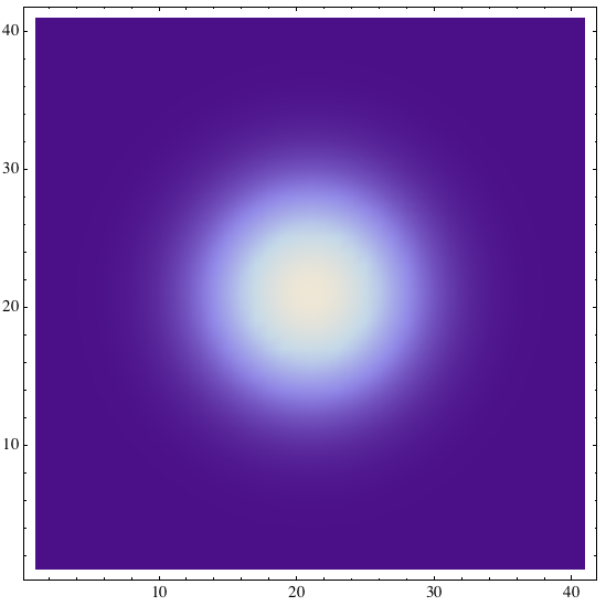
This is the ground state. The eigenvalues have near-degeneracies:

e = Eigenvalues[h, -10]

(*
==> {3.97742, 3.97742, 3.96769, 3.96769, 2.98745, 2.98244, \
2.98244, 1.99247, 1.99247, 0.997494}
*)

The exact values of the energy should be 4, 3, 2, 1 in descending order.

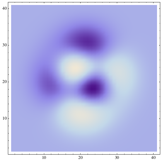
The degeneracies are the reason why for most states you get superpositions that don't look like the rotationally symmetrized Gauss-Laguerre functions of Gauss-Hermite functions - but they are valid solutions nonetheless (to within the accuracy of the discretization):

ListDensityPlot[Partition[v[[4]],2nX+1],PlotRange->All]

In the construction of h, I used a trick to compute the matrix corresponding to the Laplacian: it invokes the AdjacencyMatrix of a GridGraph. In principle, it may be better to instead use NDSolve'FiniteDifferenceDerivative for this. But I think it's a cute fact that this particular AdjacencyMatrix also works. I may get back to adding an alternative approach using the NDSolve functionality later.

This is a quick-and dirty implementation without bells and whistles, but it shows the main steps. It also shows that the boundary effects at the edge of the grid are not important as long as you only look at states that are low enough in energy so as to not reach that boundary. This is also why time-dependent wave packet solutions in the same potential can be modeled on a finite grid.

Edit

The next step is to apply the method to an anisotropic harmonic oscillator, with potential energy $V(x,y) = 1/2 (x^2 + y^2 + x y)$, as was asked for in the comments:

nX = 20;
a = .2;

Clear[v];
v[x_, y_] := 1/2 (x^2 + y^2 + x y)

vGrid = Table[v[a i, a j], {i, -nX, nX}, {j, -nX, nX}];

xyList = Tuples[Range[1, 2 nX + 1], 2];

Timing[h = 
   DiagonalMatrix[SparseArray[(vGrid[[##]] & @@@ xyList) + 2/a^2]] - 
    1/(2 a^2) AdjacencyMatrix[GridGraph[{2 nX + 1, 2 nX + 1}]];]

(* ==>{0.009491,Null}*)

v = Eigenvectors[h, -10];

ListDensityPlot[Partition[v[[10]], 2 nX + 1], PlotRange -> All]

(* ==> {0.008648, Null} *)

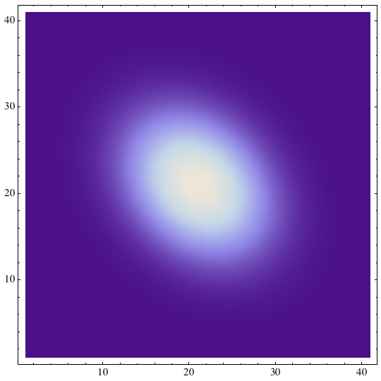
As expected, the ground state now is deformed (elliptical) and oriented along a diagonal.

Edit 2: an even more basic approach

To avoid any advanced functions that may not be present in older versions of Mathematica, here is a practically identical formulation where the finite-difference approximation is constructed in a more straight-forward (i.e. low-level) way. I'm again using the anisotropic oscillator of the last example - everything up to xyList is copied verbatim from above.

nX = 20;
a = .2;

Clear[v];
v[x_, y_] := 1/2 (x^2 + y^2 + x y)

vGrid = Table[v[a i, a j], {i, -nX, nX}, {j, -nX, nX}];

xyList = Tuples[Range[1, 2 nX + 1], 2];

ClearAll[hash];
Evaluate[hash /@ xyList] = Range[Length[xyList]];
hash[{0, n_}] := hash[{2 nX + 1, n}];
hash[{n_, 0}] := hash[{n, 2 nX + 1}];
hash[{2 nX + 2, n_}] := hash[{1, n}];
hash[{n_, 2 nX + 2}] := hash[{n, 1}];

s1 = 
  SparseArray[
   Flatten[Table[{{hash[{i, j}], hash[{i, j + 1}]} -> 
       1, {hash[{i, j}], hash[{i + 1, j}]} -> 
       1, {hash[{i, j}], hash[{i, j - 1}]} -> 
       1, {hash[{i, j}], hash[{i - 1, j}]} -> 1}, {i, 1, 
      2 nX + 1}, {j, 1, 2 nX + 1}]]];

h1 = 
  DiagonalMatrix[SparseArray[(vGrid[[##]] & @@@ xyList) + 2/a^2]] - 
   1/(2 a^2) s1;

This is the equivalent to h in the previous examples. It is the Hamiltonian matrix that will now be diagonalized to get the eigenvalues and eigenvectors:

e1 = Eigenvalues[h1, -10]

(*
==> {4.09354, 3.77227, 3.58063, 3.39729, 3.07122, 2.88156, \
2.36968, 2.1824, 1.66728, 0.963587}
*)

v1 = Eigenvectors[h1, -10];

ListDensityPlot[Partition[v1[[4]], 2 nX + 1], 
 PlotRange -> All]

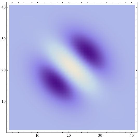
Here I chose to plot an excited state instead of the ground state because it shows nicely that after breaking the rotational symmetry we don't have degeneracies anymore and therefore get eigenfunctions that look like the expected Gauss-Hermit functions in both orthogonal directions (along the diagonals), as one would also obtain by first finding the normal modes exactly. This finite difference algorithm of course doesn't know or care about the existence of rotational symmetry or separability, so it will also work with binding potentials that are not harmonic oscillators.

Regarding three dimensions

The generalization to higher dimensions is in principle quite straightforward, but you'll have to consult some text on finite-difference methods to construct the second-derivate stencil properly. In those cases, the availability of built-in methods becomes really useful. There is a lot more to read about this in the documentation (search for FiniteDifferenceDerivative, it will in fact tell you how to construct a 2D Laplacian).

Edit to generalize my first approach to 3D

To generalize my earlier AdjacencyMatrix trick to three dimensions, you would need to calculate the Hamiltonian as follows:

h = DiagonalMatrix[SparseArray[(vGrid[[##]] & @@@ xyList) + 3/a^2]] - 
    1/(2 a^2) AdjacencyMatrix[GridGraph[{2 nX + 1, 2 nX + 1, 2 nX + 1}]]

Note the factor 3 instead of 2 in the additive constant on the diagonal. The constant on the diagonal is 1/a^2 times the number of dimensions of the grid.

The difference between using AdjacencyMatrix and the last approach is in the boundary conditions. The AdjacencyMatrix method does not implement periodic boundary conditions, whereas the last approach does. However, these boundary conditions are irrelevant in the present calculation because the bound states are assumed to not feel the boundary anyway.

I like the AdjacencyMatrix approach mainly because it is a more descriptive formulation, saying in code what the topology of the laplacian matrix really looks like.

Edit regarding grid spacing

To change the grid spacing without changing the physics, you have to keep the product a*nX large enough to ensure that the eigenstates you're interested in are not affected by the grid boundary. The value a*nX is the largest x or y coordinate that will be sampled, and your potential at those coordinates should be high enough to exclude the wave function of any relevant eigenstate from the boundary.

One could also combine this algorithm with my answer here to insure that the eigenvalues and eigenvectors are sorted in the correct way.

Edit regarding differentiation order

For completeness, and in response to the comments, I'm also listing another approach based on the built-in function NDSolve'FiniteDifferenceDerivative, which allows us to specify the differentiation order. This overcomes the limitation of the previous methods which use the lowest-order finite-difference approximation to the second derivative. Mathematica is able to generate finite-difference derivative matrices for higher order, by specifying the option "DifferenceOrder" as shown below. The value 4 is actually the default.

nX = 20;
a = .2;

Clear[v];
v[x_, y_] := 1/2 (x^2 + y^2 + x y)

vGrid = Table[v[a i, a j], {i, -nX, nX}, {j, -nX, nX}];
xRange = Range[1, 2 nX + 1];
xyList = Tuples[xRange, 2];

h2 = DiagonalMatrix[
    SparseArray[(vGrid[[##]] & @@@ xyList)]] - 
    1/(2 a^2) Sum[
     NDSolve`FiniteDifferenceDerivative[i, {xRange, xRange}, 
       "DifferenceOrder" -> 4]["DifferentiationMatrix"], 
    {i, {{2, 0}, {0, 2}}}];

{en2, ψ2} = Eigensystem[h2, -10];

ListDensityPlot[Partition[ψ2[[5]], 2 nX + 1], PlotRange -> All]

Using higher differentiation order is then simply a matter of changing the value 4 to something else, and making sure that the grid is large enough to give sensible results for that order.

This is the two-dimensional generalization of what I did in a closely related answer here.