Added appendix in response to comments.
Source Link
bobthechemist
  • 19.8k
  • 4
  • 56
  • 140

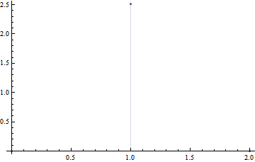
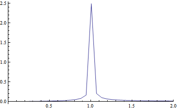
Paying close attention to the documentation for Fourier and FourierTransform one notes that the coefficients of the Sum/Integral terms are different; therefore, to obtain a discrete transform with amplitudes equal to those from the continuous transform, one must multiply the former by Sqrt[2 Pi / n] where n is the length of the dataset:

The continuous waveform:

DiscretePlot[
 Evaluate[Abs@FourierTransform[2 Sin[x], x, w] /. 
   DiracDelta -> DiscreteDelta], {w, 0, 2}]
Mathematica graphics

and the discrete waveform:

With[{datalength = 100}, 
 ListPlot[(Sqrt[2 Pi]/Sqrt[datalength]) Abs[
    Fourier[Table[2*Sin[x], {x, 0, datalength}]]], Joined -> True, 
  PlotRange -> {{0, 2}, All}, DataRange -> {0, 2Pi}]]
Mathematica graphics

Appendix: Why isn't the amplitude "right"

In the comments, the OP asks why the amplitude of the function 2 Sin[x] appears to be ~2.5 in the transformed data. Let's take a pedagogical approach here, in part to show off how one might use Mathematica to answer these types of questions on their own.

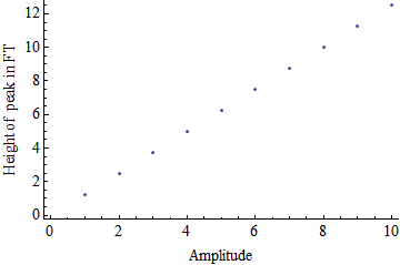
Is there a relationship between the amplitude of the wave and the height of the peak in the transform?

Hopefully, the answer is yes, but let's generate some data, plot it and see.

testdata = 
 Table[{i, 
   Evaluate[
    Abs@FourierTransform[i Sin[x], x, w] /. {DiracDelta -> 
       DiscreteDelta, w -> 1}]}, {i, 1, 10, 1}]
Mathematica graphics

There is a linear relationship - yeah! What is that relationship?

Let's perform a linear least squares analysis on testdata to see what the slope of that line is. I will assume that the plot should go through zero.

LinearModelFit[testdata, x, x]["BestFitParameters"] // Chop
(* {0, 1.25331} *)

So that means that the height of the peak in the transformed data will be 1.25331 times larger than the amplitude of the time-domain function. Where does this 1.25331 come from? Taking a closer look at testdata:

Mathematica graphics

We see a Sqrt[2 Pi]/2 nestled in there. Evaluating N@Sqrt[2 Pi]/2 yields:

(* 1.25331 *)

Nice.

Paying close attention to the documentation for Fourier and FourierTransform one notes that the coefficients of the Sum/Integral terms are different; therefore, to obtain a discrete transform with amplitudes equal to those from the continuous transform, one must multiply the former by Sqrt[2 Pi / n] where n is the length of the dataset:

The continuous waveform:

DiscretePlot[
 Evaluate[Abs@FourierTransform[2 Sin[x], x, w] /. 
   DiracDelta -> DiscreteDelta], {w, 0, 2}]

Mathematica graphics

and the discrete waveform:

With[{datalength = 100}, 
 ListPlot[(Sqrt[2 Pi]/Sqrt[datalength]) Abs[
    Fourier[Table[2*Sin[x], {x, 0, datalength}]]], Joined -> True, 
  PlotRange -> {{0, 2}, All}, DataRange -> {0, 2Pi}]]

Mathematica graphics

Appendix: Why isn't the amplitude "right"

In the comments, the OP asks why the amplitude of the function 2 Sin[x] appears to be ~2.5 in the transformed data. Let's take a pedagogical approach here, in part to show off how one might use Mathematica to answer these types of questions on their own.

Is there a relationship between the amplitude of the wave and the height of the peak in the transform?

Hopefully, the answer is yes, but let's generate some data, plot it and see.

testdata = 
 Table[{i, 
   Evaluate[
    Abs@FourierTransform[i Sin[x], x, w] /. {DiracDelta -> 
       DiscreteDelta, w -> 1}]}, {i, 1, 10, 1}]

Mathematica graphics

There is a linear relationship - yeah! What is that relationship?

Let's perform a linear least squares analysis on testdata to see what the slope of that line is. I will assume that the plot should go through zero.

LinearModelFit[testdata, x, x]["BestFitParameters"] // Chop
(* {0, 1.25331} *)

So that means that the height of the peak in the transformed data will be 1.25331 times larger than the amplitude of the time-domain function. Where does this 1.25331 come from? Taking a closer look at testdata:

Mathematica graphics

We see a Sqrt[2 Pi]/2 nestled in there. Evaluating N@Sqrt[2 Pi]/2 yields:

(* 1.25331 *)

Nice.

Source Link
bobthechemist
  • 19.8k
  • 4
  • 56
  • 140

Paying close attention to the documentation for Fourier and FourierTransform one notes that the coefficients of the Sum/Integral terms are different; therefore, to obtain a discrete transform with amplitudes equal to those from the continuous transform, one must multiply the former by Sqrt[2 Pi / n] where n is the length of the dataset:

The continuous waveform:

DiscretePlot[
 Evaluate[Abs@FourierTransform[2 Sin[x], x, w] /. 
   DiracDelta -> DiscreteDelta], {w, 0, 2}]

Mathematica graphics

and the discrete waveform:

With[{datalength = 100}, 
 ListPlot[(Sqrt[2 Pi]/Sqrt[datalength]) Abs[
    Fourier[Table[2*Sin[x], {x, 0, datalength}]]], Joined -> True, 
  PlotRange -> {{0, 2}, All}, DataRange -> {0, 2Pi}]]

Mathematica graphics