Paying close attention to the documentation for [`Fourier`](http://reference.wolfram.com/mathematica/ref/Fourier.html) and [`FourierTransform`](http://reference.wolfram.com/mathematica/ref/FourierTransform.html) one notes that the coefficients of the Sum/Integral terms are different; therefore, to obtain a discrete transform with amplitudes equal to those from the continuous transform, one must multiply the former by Sqrt[2 Pi / n] where n is the length of the dataset:
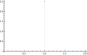
The continuous waveform:
DiscretePlot[
Evaluate[Abs@FourierTransform[2 Sin[x], x, w] /.
DiracDelta -> DiscreteDelta], {w, 0, 2}]

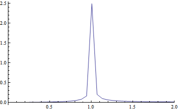
and the discrete waveform:
With[{datalength = 100},
ListPlot[(Sqrt[2 Pi]/Sqrt[datalength]) Abs[
Fourier[Table[2*Sin[x], {x, 0, datalength}]]], Joined -> True,
PlotRange -> {{0, 2}, All}, DataRange -> {0, 2Pi}]]

# Appendix: Why isn't the amplitude "right" #
In the comments, the OP asks why the amplitude of the function `2 Sin[x]` appears to be ~2.5 in the transformed data. Let's take a pedagogical approach here, in part to show off how one might use Mathematica to answer these types of questions on their own.
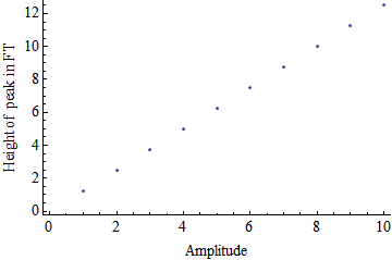
**Is there a relationship between the amplitude of the wave and the height of the peak in the transform?**
Hopefully, the answer is yes, but let's generate some data, plot it and see.
testdata =
Table[{i,
Evaluate[
Abs@FourierTransform[i Sin[x], x, w] /. {DiracDelta ->
DiscreteDelta, w -> 1}]}, {i, 1, 10, 1}]

**There is a linear relationship - yeah! What is that relationship?**
Let's perform a linear least squares analysis on `testdata` to see what the slope of that line is. I will assume that the plot should go through zero.
LinearModelFit[testdata, x, x]["BestFitParameters"] // Chop
(* {0, 1.25331} *)
So that means that the height of the peak in the transformed data will be 1.25331 times larger than the amplitude of the time-domain function. Where does this 1.25331 come from? Taking a closer look at `testdata`:

We see a Sqrt[2 Pi]/2 nestled in there. Evaluating `N@Sqrt[2 Pi]/2` yields:
(* 1.25331 *)
Nice.