Character edge finding

Question

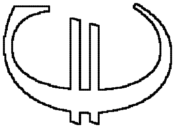
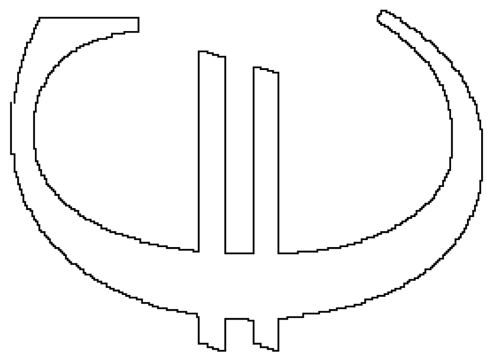
The following line of code finds the edge of a character:

pic = Binarize[GradientFilter[Rasterize[Style["\[Euro]", FontFamily -> "Times"], 
                              ImageSize -> 200] // Image, 1]]

The coordinates of the edges can be found as follows:

pdata = Position[ImageData[pic], 1];

Test:

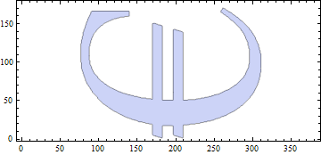
Graphics[Point[pdata]]

However, the points are not sorted in an order usable by Line or Polygon:

Graphics[Polygon[pdata]]

This brings me to my question:

• What would be an efficient method to sort the coordinates so that it would plot properly with Line or Polygon?

Additionally,

• How to thin and smooth the set of points?
• How to deal with characters with holes in them, like the ones below?

or

Answer 1

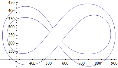
I think there is a neat solution. We have curios function ListCurvePathPlot:

pic = Thinning@Binarize[GradientFilter[Rasterize[Style["\[Euro]", 
FontFamily -> "Times"], ImageSize -> 200] // Image, 1]];

pdata = Position[ImageData[pic], 1];

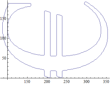
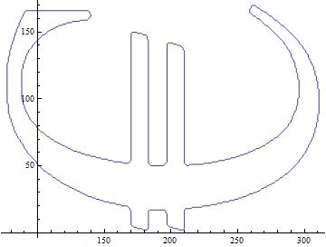
lcp = ListCurvePathPlot[pdata]

Now this is of course Graphics containing Line with set of points

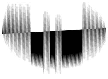
lcp[[1, 1, 3, 2]]

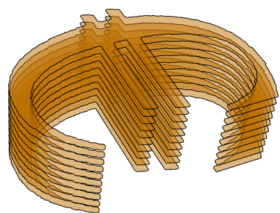
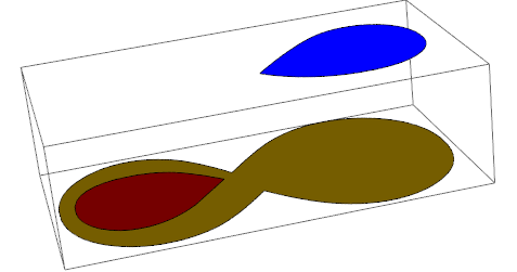
So of course we can do something like

Graphics3D[Table[{Orange, Opacity[.5],Polygon[(#~Join~{10 n})&
/@ lcp[[1, 1, 3, 2, 1]]]}, {n, 10}], Boxed -> False]

I think it works nicely with "8" and Polygon:

pic = Thinning@Binarize[GradientFilter[
Rasterize[Style["8", FontFamily -> "Times"], ImageSize -> 500] //Image, 1]]; 
pdata = Position[ImageData[pic], 1]; lcp = ListCurvePathPlot[pdata]

And you can do polygons 1-by-1 extraction:

Graphics3D[{{Orange, Thick, Polygon[(#~Join~{0}) & /@ lcp[[1, 1, 3, 2, 1]]]},
  {Red, Thick, Polygon[(#~Join~{1}) & /@ lcp[[1, 1, 3, 3, 1]]]},
  {Blue, Thick, Polygon[(#~Join~{200}) & /@ lcp[[1, 1, 3, 4, 1]]]}}]

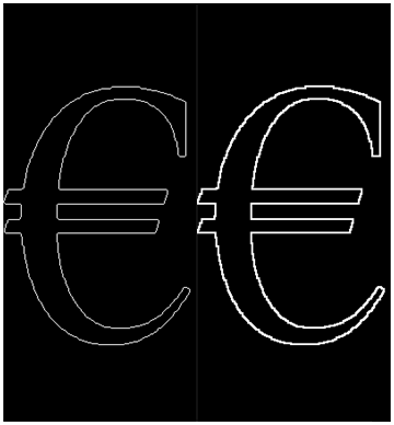
=> To smooth the curve set ImageSize -> "larger number" in your pic = code.

=> To thin the curve to 1 pixel wide use Thinning:

 Row@{Thinning[#], Identity[#]} &@Binarize[GradientFilter[
 Rasterize[Style["\[Euro]", FontFamily -> "Times"], 
 ImageSize -> 200] // Image, 1]]

You can do curve extraction more efficiently with Mathematica. A simple example would be

text = First[
   First[ImportString[
     ExportString[
      Style["\[Euro] 9 M-8 ", Italic, FontSize -> 24, 
       FontFamily -> "Times"], "PDF"], "PDF", 
     "TextMode" -> "Outlines"]]];

Graphics[{EdgeForm[Black], FaceForm[], text}]

Answer 2

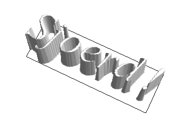
Possible answer using ClusteringComponents:

image=Rasterize[
 Style["Sjoerd!",Italic,FontSize->24,FontFamily->"Times"],
 "Image",ImageSize->200]

cluster=ClusteringComponents[ImageReflect[image,Left->Right]];

ListPlot3D[cluster,Mesh->False,BoxRatios->{3,1,1},Boxed->False,
 Axes->False,Lighting->"Neutral",
 ViewPoint->{-0.4340374864952124,0.8958897046884841,3.2340366567727856`}]

Another fun one, using RegionPlot3D on the same cluster data:

RegionPlot3D[
 cluster[[Round[x], Round[y]]] > 1.5, {x, 1, 66}, {y, 1, 202}, {z, 0, 1}, 
 PlotPoints -> 80, Mesh -> False, Axes -> False, Boxed -> False, 
 Lighting -> "Neutral"]

Answer 3

You can recast this to a problem of finding a Hamiltonian cycle in a graph constructed in a certain way from your points (distance graph). First, compute mutual distances:

distances = 
With[{tr = Transpose[N@pdata]},
 Function[point, Sqrt[Total[(point - tr)^2]]] /@ 
  N[pdata]];

Now, construct an adjacency matrix by stating that two vertices (points) are connected if their disctance is smaller than a certain radius (which I tweaked a bit):

radius = 1;
adj = Unitize@Clip[distances, {0, radius}, {0, 0}];

Now build an adjacency graph:

graph = AdjacencyGraph[adj];

And find the cycle:

cycle = FindHamiltonianCycle[graph];

Finally, the plot:

Graphics[Polygon[pdata[[cycle[[1, All, 1]]]]]]

This probably can be refined further.

Answer 4

I tried FindCurvePath and FindShortestTour, but didn't succeed. The latter is too slow to finish on my machine, except when using the "Greedy" method, which does not give a perfect solution.

Here's something different:

matrix = Rasterize[
    Style["\[Euro]", FontFamily -> "Times", Antialiasing -> False], 
    "Data", ImageSize -> 200][[All, All, 1]];

fun = ListInterpolation[matrix]

{{xmin, xmax}, {ymin, ymax}} = fun["Domain"]

g = RegionPlot[fun[x, y] < 128, {x, xmin, xmax}, {y, ymin, ymax}, 
 PlotPoints -> 50, AspectRatio -> Automatic]

The filling of the region is made of a large number of polygons, but the outline is just one or more lines, which we can easily extract ...

Graphics[Cases[Normal[g], Line[___], Infinity]]

... or even make into polygons again:

% /. Line -> Polygon

---

EDIT

I noticed Vitaliy's Thinning solution. With that ListCurvePathPlot works:

img = Thinning@
  EdgeDetect@
   Rasterize[Style["\[Euro]", FontFamily -> "Times"], "Image", 
    ImageSize -> 200]

points = N@Position[ImageData[img], 1];

ListCurvePathPlot[points]

FindCurvePath will give you the ordering of points. This won't of course work for the image of number 8 or 9.

We can also apply a slight smoothing:

orderedPoints = points[[First@FindCurvePath[points]]];    
ListLinePlot[MovingAverage[orderedPoints, 3]]

Warning: FindCurvePath may return a number of disconnected curves!

Answer 5

A year late, but here are my thoughts:

As Szabolcs showed, extracting the Line primitives from a RegionPlot provides a convenient way to produce a polygon from an image. The function imgToPolys below does just that - it's essentially the same as Szabolcs' code but I use ImageValue instead of creating an interpolating function from the image data.

Of course, some of the polygons produced this way are the "holes" in letters. In order to display the text properly we need to identify which polygons are holes and which are "solids" (for want of a better word). The function findHoles takes a list of polygons and uses the undocumented function Graphics`Mesh`InPolygonQ to test whether the first point of each polygon lies inside any of the other polygons. I've assumed that any "holes" are completely contained within a surrounding "solid", so that testing a single point is sufficient. The expression returned by findHoles is a list of {solids, holes}.

imgToPolys[img_Image] :=
 Module[{w, h, rp},
  {w, h} = ImageDimensions[img];
  rp = RegionPlot[
    ImageValue[img, {x, y}] < 0.5, {x, 0.5, w - 0.5}, {y, 0.5, h - 0.5}, 
    PlotPoints -> 100];
  Cases[Normal[rp], l_Line :> Polygon @@ l, -1]];

findHoles[p : {_Polygon ..}] := Module[{inq, holes, solids},
  inq = Outer[Graphics`Mesh`InPolygonQ, p, p[[All, 1, 1]], 1];
  holes = DeleteCases[inq ~Position~ True , {x_, x_}][[All, 2]];
  solids = Complement[Range[Length[p]], holes];
  {p[[solids]], p[[holes]]}];

Here's an example where I have shown the holes in white, so they look like, well, holes.

input = Style["{##}&/@", Bold, FontFamily -> "Calibri", FontSize -> 12];

img = Rasterize[input, ImageSize -> 800] ~ColorConvert~ "Grayscale" ~
  ImageResize~ 400;

{solids, holes} = findHoles@imgToPolys@img;

Graphics[{EdgeForm[Red], Yellow, solids, White, holes}]

Faster method using FilledCurve

The procedure above is rather slow, due to the RegionPlot. An alternative way to create polygons from text is from the FilledCurve primitives that can be obtained by converting via PDF (as in Vitaliy's answer). Below is some code to convert the filled curves into polygons.

The conversion is a two stage process, first the filled curves are converted to bezier curves, then the bezier curves are sampled at some number of points (default 10), and the coordinates fed into a Polygon expression.

As previously, the polygons can then be split into "solids" and "holes" using findHoles.

filledCurveToBeziers[fc_FilledCurve] := MapThread[processFCdata, List @@ fc];

processFCdata[desc_, pts_] := Module[{r, sd},
  r = Range @@@ 
    ReplacePart[
     Partition[Prepend[Accumulate[desc[[All, 2]]], 0], 2, 1], {1, 1} -> 1];
  sd = desc[[All, 3]] /. {0 -> 1};
  MapThread[BezierCurve[pts[[#1]], SplineDegree -> #2] &, {r, sd}]];

beziersToPolygons[x_, n_: 10] :=
 Module[{samples},
  samples = x /. BezierCurve[data__] :> BezierFunction[data] /@ Range[0, 1, 1/n];
  Polygon /@ Select[Split[Flatten[#, 1]][[All, 1]] & /@ samples, Length[#] > 1 &]];

This approach is much faster, since it completely avoids the rasterization and image processing.

{solids, holes} = 
  With[{fc = Cases[ImportString[ExportString[input, "PDF"]], _FilledCurve, -1]},
   Transpose[findHoles@beziersToPolygons[filledCurveToBeziers@#, 10] & /@ fc]];

Graphics[{EdgeForm[Red], Yellow, solids, White, holes}]

Answer 6

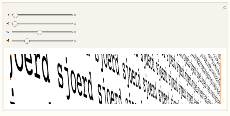
From the sublime to the ridiculous. By way of contrast, here's another approach to 3D text rendering:

sjoerd = Image[
     Rasterize[" sjoerd ", RasterSize -> 900, ImageSize -> 900]];

Manipulate[
   ImagePerspectiveTransformation[sjoerd, 
      ScalingMatrix[s, {v1, v2, v3}],  Padding -> "Periodic", 
      Resampling -> "Bicubic"], {{s, .2}, 0.1, 8}, 
         {{v1, -1}, -1, 1}, {{v2, -0.1}, -1, 1}, {{v3, .3}, 0.1, 1}] 

Perhaps it's more fun to play with than to look at... :)

Answer 7

Posting as an answer per request. See

http://forums.wolfram.com/mathgroup/archive/2011/Mar/msg00529.html

Caveat: It's been almost a year since I've toyed with that code. Strange things can happen to code left on the dusty shelves of Usenet. The basic idea was similar to Leonid's: use some proximity measure to find neighbor pairs. And be prepared for some failure cases that may need further tweaking, that is to say, segment "jumps" to nearby lines.