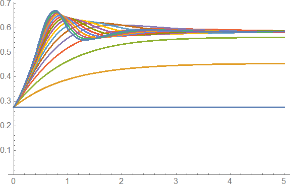
Waiting some time for a straightforward numerical answer, here my attempt, which assumes \[Beta] = 1 (without loss of generality) and predefined values c0==0.2,T0==5 :
c0 = 2/10; T = 5;
gip[eps_] :=Module[{x, t},
Interpolation[Table[{t,eps[t]^2 + c0 + Exp[-t] NIntegrate[eps[s] Exp[s], {s, 0, t}] -Exp[-t] (1 + eps[t]) NIntegrate[eps[s]^2 Exp[s], {s, 0, t}]}, {t, Subdivide[0, T, 25]}]]]
Function gip get's a pure function as input argument and returns an InterpolationFunction, which might be used iteratively.
solm = NestList[gip, 1/2 (1 - Sqrt[1 - 4 c0]) &, 15] ;
Plot[Evaluate[Through[solm [t]]], {t, 0, T}, PlotRange -> {0, All}]
The solution doesn't match completely @cesaro's one (shows superimposed oscillations). Perhaps it shows a first step for a completely numerical solution.
To exclude the influence of simple Interpolation I also tried a numerical solution using NDSolveValue:
ff = Function[{t},
NDSolveValue[{i1'[t] == #[t] Exp[t], i1[0] == 0,i2'[t] == #[t]^2 Exp[t], i2[0] == 0},#[t]^2 + c0 + Exp[-t] (i1[t] - (1 + #[t]) i2[t])
, {t, 0,T}, DependentVariables -> {i1, i2},Method -> {Automatic ,"DiscontinuityProcessing" -> False  } ,AccuracyGoal -> 10 ]] & ;
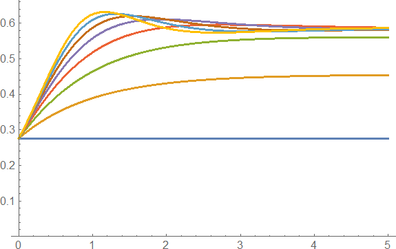
which gives the same result(I used only 7 iterations because of increased evaluation time):
sol = NestList[ff, 1/2 (1 - Sqrt[1 - 4 c0]) &, 7]; // AbsoluteTiming
Plot[Evaluate[Through[sol[t]]], {t, 0, T}, PlotRange -> {0, All}]
Hints for improvement are welcome!


