added 17 characters in body
Source Link
Ulrich Neumann
  • 56.8k
  • 2
  • 26
  • 60

Waiting some time for a straightforward numerical answer, here my attempt, which assumes \[Beta] = 1 (without loss of generality) and predefined values c0==0.2,T0==5 :

c0 = 2/10; T = 5;
gip[eps_] :=Module[{x, t}, 
Interpolation[Table[{t,eps[t]^2 + c0 + Exp[-t] NIntegrate[eps[s] Exp[s], {s, 0, t}] -Exp[-t] (1 + eps[t]) NIntegrate[eps[s]^2 Exp[s], {s, 0, t}]}, {t, Subdivide[0, T, 25]}]]] 

Function gip get's a pure function as input argument and returns an InterpolationFunction, which might be used iteratively.

With appropriate starting value eps[0]== 1/2 (1 - Sqrt[1 - 4 c0]) (second solution branch eps[0]== 1/2 (1 + Sqrt[1 - 4 c0]) omitted ) it follows

solm = NestList[gip, 1/2 (1 - Sqrt[1 - 4 c0]) &, 15] ;
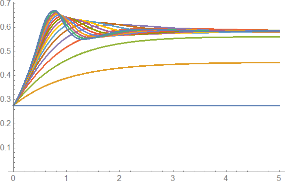
Plot[Evaluate[Through[solm [t]]], {t, 0, T}, PlotRange -> {0, All}]

enter image description here

The solution doesn't match completely @cesaro's one (shows superimposed oscillations). Perhaps it shows a first step for a completely numerical solution.

To exclude the influence of simple Interpolation I also tried a numerical solution using NDSolveValue (substitution i1[t]==Integrate[eps[s]Exp[s],{s,0,t}] and i2[t]==Integrate[eps[s]^2 Exp[s],{s,0,t}]) :

ff = Function[{t}, 
NDSolveValue[{i1'[t] == #[t] Exp[t], i1[0] == 0, 
i2'[t] == #[t]^2 Exp[t], i2[0] == 0}, 
#[t]^2 + c0 + Exp[-t] (i1[t] - (1 + #[t]) i2[t]) 
, {t, 0,T}, DependentVariables -> {i1, i2} 
,Method -> {Automatic ,"DiscontinuityProcessing" -> False  } ,AccuracyGoal -> 10 ]] & ;

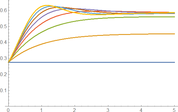
which gives the same result(I used only 7 iterations because of increased evaluation time):

sol = NestList[ff, 1/2 (1 - Sqrt[1 - 4 c0]) &, 7]; // AbsoluteTiming 
Plot[Evaluate[Through[sol[t]]], {t, 0, T}, PlotRange -> {0, All}]

enter image description here

conclusion

The two numerical solutions, obtained with two independent methods, match very well. I'm quite convinced that the solutions describe the iteration of the given integral equation.

Hints for improvement are welcome!

Waiting some time for a straightforward numerical answer, here my attempt, which assumes \[Beta] = 1 (without loss of generality) and predefined values c0==0.2,T0==5 :

c0 = 2/10; T = 5;
gip[eps_] :=Module[{x, t}, 
Interpolation[Table[{t,eps[t]^2 + c0 + Exp[-t] NIntegrate[eps[s] Exp[s], {s, 0, t}] -Exp[-t] (1 + eps[t]) NIntegrate[eps[s]^2 Exp[s], {s, 0, t}]}, {t, Subdivide[0, T, 25]}]]] 

Function gip get's a pure function as input argument and returns an InterpolationFunction, which might be used iteratively.

With appropriate starting value eps[0]== 1/2 (1 - Sqrt[1 - 4 c0]) (second solution branch eps[0]== 1/2 (1 + Sqrt[1 - 4 c0]) omitted ) it follows

solm = NestList[gip, 1/2 (1 - Sqrt[1 - 4 c0]) &, 15] ;
Plot[Evaluate[Through[solm [t]]], {t, 0, T}, PlotRange -> {0, All}]

enter image description here

The solution doesn't match completely @cesaro's one (shows superimposed oscillations). Perhaps it shows a first step for a completely numerical solution.

To exclude the influence of simple Interpolation I also tried a numerical solution using NDSolveValue (substitution i1[t]==Integrate[eps[s]Exp[s],{s,0,t}] and i2[t]==Integrate[eps[s]^2 Exp[s],{s,0,t}]) :

ff = Function[{t}, 
NDSolveValue[{i1'[t] == #[t] Exp[t], i1[0] == 0,i2'[t] == #[t]^2 Exp[t], i2[0] == 0},#[t]^2 + c0 + Exp[-t] (i1[t] - (1 + #[t]) i2[t]) 
, {t, 0,T}, DependentVariables -> {i1, i2},Method -> {Automatic ,"DiscontinuityProcessing" -> False  } ,AccuracyGoal -> 10 ]] & ;

which gives the same result(I used only 7 iterations because of increased evaluation time):

sol = NestList[ff, 1/2 (1 - Sqrt[1 - 4 c0]) &, 7]; // AbsoluteTiming 
Plot[Evaluate[Through[sol[t]]], {t, 0, T}, PlotRange -> {0, All}]

enter image description here

conclusion

The two numerical solutions, obtained with two independent methods, match very well. I'm quite convinced that the solutions describe the iteration of the given integral equation.

Hints for improvement are welcome!
Waiting some time for a straightforward numerical answer, here my attempt, which assumes \[Beta] = 1 (without loss of generality) and predefined values c0==0.2,T0==5 :

c0 = 2/10; T = 5;
gip[eps_] :=Module[{x, t}, 
Interpolation[Table[{t,eps[t]^2 + c0 + Exp[-t] NIntegrate[eps[s] Exp[s], {s, 0, t}] -Exp[-t] (1 + eps[t]) NIntegrate[eps[s]^2 Exp[s], {s, 0, t}]}, {t, Subdivide[0, T, 25]}]]] 

Function gip get's a pure function as input argument and returns an InterpolationFunction, which might be used iteratively.

With appropriate starting value eps[0]== 1/2 (1 - Sqrt[1 - 4 c0]) (second solution branch eps[0]== 1/2 (1 + Sqrt[1 - 4 c0]) omitted ) it follows

solm = NestList[gip, 1/2 (1 - Sqrt[1 - 4 c0]) &, 15] ;
Plot[Evaluate[Through[solm [t]]], {t, 0, T}, PlotRange -> {0, All}]

enter image description here

The solution doesn't match completely @cesaro's one (shows superimposed oscillations). Perhaps it shows a first step for a completely numerical solution.

To exclude the influence of simple Interpolation I also tried a numerical solution using NDSolveValue (substitution i1[t]==Integrate[eps[s]Exp[s],{s,0,t}] and i2[t]==Integrate[eps[s]^2 Exp[s],{s,0,t}]) :

ff = Function[{t}, 
NDSolveValue[{i1'[t] == #[t] Exp[t], i1[0] == 0, 
i2'[t] == #[t]^2 Exp[t], i2[0] == 0}, 
#[t]^2 + c0 + Exp[-t] (i1[t] - (1 + #[t]) i2[t]) 
, {t, 0,T}, DependentVariables -> {i1, i2} 
,Method -> {Automatic ,"DiscontinuityProcessing" -> False  },AccuracyGoal -> 10 ]] & ;

which gives the same result(I used only 7 iterations because of increased evaluation time):

sol = NestList[ff, 1/2 (1 - Sqrt[1 - 4 c0]) &, 7]; // AbsoluteTiming 
Plot[Evaluate[Through[sol[t]]], {t, 0, T}, PlotRange -> {0, All}]

enter image description here

conclusion

The two numerical solutions, obtained with two independent methods, match very well. I'm quite convinced that the solutions describe the iteration of the given integral equation.

Hints for improvement are welcome!
added 105 characters in body
Source Link
Ulrich Neumann
  • 56.8k
  • 2
  • 26
  • 60

Waiting some time for a straightforward numerical answer, here my attempt, which assumes \[Beta] = 1 (without loss of generality) and predefined values c0==0.2,T0==5 :

c0 = 2/10; T = 5;
gip[eps_] :=Module[{x, t}, 
Interpolation[Table[{t,eps[t]^2 + c0 + Exp[-t] NIntegrate[eps[s] Exp[s], {s, 0, t}] -Exp[-t] (1 + eps[t]) NIntegrate[eps[s]^2 Exp[s], {s, 0, t}]}, {t, Subdivide[0, T, 25]}]]] 

Function gip get's a pure function as input argument and returns an InterpolationFunction, which might be used iteratively.

With appropriate starting value eps[0]== 1/2 (1 - Sqrt[1 - 4 c0]) (second solution branch eps[0]== 1/2 (1 + Sqrt[1 - 4 c0]) omitted ) it follows

solm = NestList[gip, 1/2 (1 - Sqrt[1 - 4 c0]) &, 15] ;
Plot[Evaluate[Through[solm [t]]], {t, 0, T}, PlotRange -> {0, All}]

enter image description here

The solution doesn't match completely @cesaro's one (shows superimposed oscillations). Perhaps it shows a first step for a completely numerical solution.

To exclude the influence of simple Interpolation I also tried a numerical solution using NDSolveValue (substitution i1[t]==Integrate[eps[s]Exp[s],{s,0,t}] and i2[t]==Integrate[eps[s]^2 Exp[s],{s,0,t}]) :

ff = Function[{t}, 
NDSolveValue[{i1'[t] == #[t] Exp[t], i1[0] == 0,i2'[t] == #[t]^2 Exp[t], i2[0] == 0},#[t]^2 + c0 + Exp[-t] (i1[t] - (1 + #[t]) i2[t]) 
, {t, 0,T}, DependentVariables -> {i1, i2},Method -> {Automatic ,"DiscontinuityProcessing" -> False  } ,AccuracyGoal -> 10 ]] & ;

which gives the same result(I used only 7 iterations because of increased evaluation time):

sol = NestList[ff, 1/2 (1 - Sqrt[1 - 4 c0]) &, 7]; // AbsoluteTiming 
Plot[Evaluate[Through[sol[t]]], {t, 0, T}, PlotRange -> {0, All}]

enter image description here

conclusion

The two numerical solutions, obtained with two independent methods, match very well. I'm quite convinced that the solutions describe the iteration of the given integral equation.

Hints for improvement are welcome!

Waiting some time for a straightforward numerical answer, here my attempt, which assumes \[Beta] = 1 (without loss of generality) and predefined values c0==0.2,T0==5 :

c0 = 2/10; T = 5;
gip[eps_] :=Module[{x, t}, 
Interpolation[Table[{t,eps[t]^2 + c0 + Exp[-t] NIntegrate[eps[s] Exp[s], {s, 0, t}] -Exp[-t] (1 + eps[t]) NIntegrate[eps[s]^2 Exp[s], {s, 0, t}]}, {t, Subdivide[0, T, 25]}]]] 

Function gip get's a pure function as input argument and returns an InterpolationFunction, which might be used iteratively.

With appropriate starting value eps[0]== 1/2 (1 - Sqrt[1 - 4 c0]) (second solution branch eps[0]== 1/2 (1 + Sqrt[1 - 4 c0]) omitted ) it follows

solm = NestList[gip, 1/2 (1 - Sqrt[1 - 4 c0]) &, 15] ;
Plot[Evaluate[Through[solm [t]]], {t, 0, T}, PlotRange -> {0, All}]

enter image description here

The solution doesn't match completely @cesaro's one (shows superimposed oscillations). Perhaps it shows a first step for a completely numerical solution.

To exclude the influence of simple Interpolation I also tried a numerical solution using NDSolveValue:

ff = Function[{t}, 
NDSolveValue[{i1'[t] == #[t] Exp[t], i1[0] == 0,i2'[t] == #[t]^2 Exp[t], i2[0] == 0},#[t]^2 + c0 + Exp[-t] (i1[t] - (1 + #[t]) i2[t]) 
, {t, 0,T}, DependentVariables -> {i1, i2},Method -> {Automatic ,"DiscontinuityProcessing" -> False  } ,AccuracyGoal -> 10 ]] & ;

which gives the same result(I used only 7 iterations because of increased evaluation time):

sol = NestList[ff, 1/2 (1 - Sqrt[1 - 4 c0]) &, 7]; // AbsoluteTiming 
Plot[Evaluate[Through[sol[t]]], {t, 0, T}, PlotRange -> {0, All}]

enter image description here

conclusion

The two numerical solutions, obtained with two independent methods, match very well. I'm quite convinced that the solutions describe the iteration of the given integral equation.

Hints for improvement are welcome!

Waiting some time for a straightforward numerical answer, here my attempt, which assumes \[Beta] = 1 (without loss of generality) and predefined values c0==0.2,T0==5 :

c0 = 2/10; T = 5;
gip[eps_] :=Module[{x, t}, 
Interpolation[Table[{t,eps[t]^2 + c0 + Exp[-t] NIntegrate[eps[s] Exp[s], {s, 0, t}] -Exp[-t] (1 + eps[t]) NIntegrate[eps[s]^2 Exp[s], {s, 0, t}]}, {t, Subdivide[0, T, 25]}]]] 

Function gip get's a pure function as input argument and returns an InterpolationFunction, which might be used iteratively.

With appropriate starting value eps[0]== 1/2 (1 - Sqrt[1 - 4 c0]) (second solution branch eps[0]== 1/2 (1 + Sqrt[1 - 4 c0]) omitted ) it follows

solm = NestList[gip, 1/2 (1 - Sqrt[1 - 4 c0]) &, 15] ;
Plot[Evaluate[Through[solm [t]]], {t, 0, T}, PlotRange -> {0, All}]

enter image description here

The solution doesn't match completely @cesaro's one (shows superimposed oscillations). Perhaps it shows a first step for a completely numerical solution.

To exclude the influence of simple Interpolation I also tried a numerical solution using NDSolveValue (substitution i1[t]==Integrate[eps[s]Exp[s],{s,0,t}] and i2[t]==Integrate[eps[s]^2 Exp[s],{s,0,t}]) :

ff = Function[{t}, 
NDSolveValue[{i1'[t] == #[t] Exp[t], i1[0] == 0,i2'[t] == #[t]^2 Exp[t], i2[0] == 0},#[t]^2 + c0 + Exp[-t] (i1[t] - (1 + #[t]) i2[t]) 
, {t, 0,T}, DependentVariables -> {i1, i2},Method -> {Automatic ,"DiscontinuityProcessing" -> False  } ,AccuracyGoal -> 10 ]] & ;

which gives the same result(I used only 7 iterations because of increased evaluation time):

sol = NestList[ff, 1/2 (1 - Sqrt[1 - 4 c0]) &, 7]; // AbsoluteTiming 
Plot[Evaluate[Through[sol[t]]], {t, 0, T}, PlotRange -> {0, All}]

enter image description here

conclusion

The two numerical solutions, obtained with two independent methods, match very well. I'm quite convinced that the solutions describe the iteration of the given integral equation.

Hints for improvement are welcome!

added 200 characters in body
Source Link
Ulrich Neumann
  • 56.8k
  • 2
  • 26
  • 60

Waiting some time for a straightforward numerical answer, here my attempt, which assumes \[Beta] = 1 (without loss of generality) and predefined values c0==0.2,T0==5 :

c0 = 2/10; T = 5;
gip[eps_] :=Module[{x, t}, 
Interpolation[Table[{t,eps[t]^2 + c0 + Exp[-t] NIntegrate[eps[s] Exp[s], {s, 0, t}] -Exp[-t] (1 + eps[t]) NIntegrate[eps[s]^2 Exp[s], {s, 0, t}]}, {t, Subdivide[0, T, 25]}]]] 

Function gip get's a pure function as input argument and returns an InterpolationFunction, which might be used iteratively.

With appropriate starting value eps[0]== 1/2 (1 - Sqrt[1 - 4 c0]) (second solution branch eps[0]== 1/2 (1 + Sqrt[1 - 4 c0]) omitted ) it follows

solm = NestList[gip, 1/2 (1 - Sqrt[1 - 4 c0]) &, 15] ;
Plot[Evaluate[Through[solm [t]]], {t, 0, T}, PlotRange -> {0, All}]

enter image description here

The solution doesn't match completely @cesaro's one (shows superimposed oscillations). Perhaps it shows a first step for a completely numerical solution.

To exclude the influence of simple Interpolation I also tried a numerical solution using NDSolveValue:

ff = Function[{t}, 
NDSolveValue[{i1'[t] == #[t] Exp[t], i1[0] == 0,i2'[t] == #[t]^2 Exp[t], i2[0] == 0},#[t]^2 + c0 + Exp[-t] (i1[t] - (1 + #[t]) i2[t]) 
, {t, 0,T}, DependentVariables -> {i1, i2},Method -> {Automatic ,"DiscontinuityProcessing" -> False  } ,AccuracyGoal -> 10 ]] & ;

which gives the same result(I used only 7 iterations because of increased evaluation time):

sol = NestList[ff, 1/2 (1 - Sqrt[1 - 4 c0]) &, 7]; // AbsoluteTiming 
Plot[Evaluate[Through[sol[t]]], {t, 0, T}, PlotRange -> {0, All}]

enter image description here

conclusion

The two numerical solutions, obtained with two independent methods, match very well. I'm quite convinced that the solutions describe the iteration of the given integral equation.

Hints for improvement are welcome!

Waiting some time for a straightforward numerical answer, here my attempt, which assumes \[Beta] = 1 (without loss of generality) and predefined values c0==0.2,T0==5 :

c0 = 2/10; T = 5;
gip[eps_] :=Module[{x, t}, 
Interpolation[Table[{t,eps[t]^2 + c0 + Exp[-t] NIntegrate[eps[s] Exp[s], {s, 0, t}] -Exp[-t] (1 + eps[t]) NIntegrate[eps[s]^2 Exp[s], {s, 0, t}]}, {t, Subdivide[0, T, 25]}]]] 

Function gip get's a pure function as input argument and returns an InterpolationFunction, which might be used iteratively.

With appropriate starting value eps[0]== 1/2 (1 - Sqrt[1 - 4 c0]) (second solution branch eps[0]== 1/2 (1 + Sqrt[1 - 4 c0]) omitted ) it follows

solm = NestList[gip, 1/2 (1 - Sqrt[1 - 4 c0]) &, 15] ;
Plot[Evaluate[Through[solm [t]]], {t, 0, T}, PlotRange -> {0, All}]

enter image description here

The solution doesn't match completely @cesaro's one (shows superimposed oscillations). Perhaps it shows a first step for a completely numerical solution.

To exclude the influence of simple Interpolation I also tried a numerical solution using NDSolveValue:

ff = Function[{t}, 
NDSolveValue[{i1'[t] == #[t] Exp[t], i1[0] == 0,i2'[t] == #[t]^2 Exp[t], i2[0] == 0},#[t]^2 + c0 + Exp[-t] (i1[t] - (1 + #[t]) i2[t]) 
, {t, 0,T}, DependentVariables -> {i1, i2},Method -> {Automatic ,"DiscontinuityProcessing" -> False  } ,AccuracyGoal -> 10 ]] & ;

which gives the same result(I used only 7 iterations because of increased evaluation time):

sol = NestList[ff, 1/2 (1 - Sqrt[1 - 4 c0]) &, 7]; // AbsoluteTiming 
Plot[Evaluate[Through[sol[t]]], {t, 0, T}, PlotRange -> {0, All}]

enter image description here

conclusion

The two numerical solutions, obtained with two independent methods, match very well. I'm quite convinced that the solutions describe the iteration of the given integral equation.

Hints for improvement are welcome!

added 10 characters in body
Source Link
Ulrich Neumann
  • 56.8k
  • 2
  • 26
  • 60
Loading
added 65 characters in body
Source Link
Ulrich Neumann
  • 56.8k
  • 2
  • 26
  • 60
Loading
added 65 characters in body
Source Link
Ulrich Neumann
  • 56.8k
  • 2
  • 26
  • 60
Loading
added 595 characters in body
Source Link
Ulrich Neumann
  • 56.8k
  • 2
  • 26
  • 60
Loading
Source Link
Ulrich Neumann
  • 56.8k
  • 2
  • 26
  • 60
Loading