Update: I misread the OP and counted the six distinct function for $k(x)$ as solutions. The OP was trying to solve equations of the form $k(x) = k_0$,
for which I get only three solutions for $0 < k_0 < \pi$, just as expected. ContourPlot has a rather weak ability to resolve roots/curves that are close together. It detects solutions via sign changes, and to detect a pair of roots it has to sample the function between them; otherwise, there would be no sign change and ContourPlot will assume there are no solutions there.
I proposed the NDSolve method below as an alternative to ContourPlot. One can use the power of NSolve to resolve the roots, and NDSolve can trace roots throughout the domain. If preferred, one could switch the dependent and independent variables and solve for x[k] as a function of k. There is a discontinuity at k = Pi/2 and one would have to solve twice, once for each of the domains 0 < k < Pi/2 and Pi/2 < k < Pi (or one could integrate over {x, 0, 2 Pi} and use Mod[x, Pi] to construct the solutions over the lower domain.
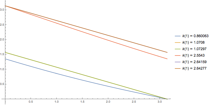
I find six distinct solutions functions $k(x)$ for T = 1/10 at high working precision:
eq[x_, k_, T_] := -Sin[3*k + x]/Sin[2*k + x] + z + 2*Cos[k] +
    T^2 + (A*T^2*Sin[k]^2)/(Sin[2*k + x]^2 + B*T^4*Sin[k]^2) /.
    {A -> 1/2, B -> 1/100000, z -> -237/100};
x0 = 1;
wp = 100;   (* working precision *)
k0 = k /. NSolve[{eq[x, k, 1/10] == 0 /. x -> x0, 0 < k < Pi},  (* six roots *)
    k, WorkingPrecision -> wp];
Quiet[
  ndsol = First@NDSolve[{
        D[eq[x, k[x], 1/10], x] == 0,
        k[x0] == #},
       k, {x, 0, Pi},
       PrecisionGoal -> 20, WorkingPrecision -> wp] & /@ k0,
  {Power::infy, Infinity::indet}];
k["Domain"] /. ndsol // N
(*  messages Power::infy, Infinity::indet, NDSolve::ndsz,... omitted  *)
(*  Domains of solutions:
  {{{0., 3.14159}}, {{0., 3.14159}}, {{0., 3.14159}},
   {{8.10181*10^-99, 3.14159}}, {{4.85285*10^-55, 3.14159}},
   {{7.61263*10^-99, 3.14159}}}
*)

ListLinePlot[k /. ndsol, PlotLegends -> Thread[k[x0] == N@k0], ImageSize -> Large]
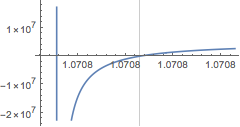
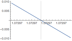
Two pair are close to each other but distinct. For instance:
ListLinePlot[
 Table[
  eq[1, k, 1/10], {k, k0[[2]] - 1*^-7, k0[[2]] + 1*^-7, 1*^-9}],
 GridLines -> {k0, None},
 DataRange -> {k0[[2]] - 1*^-7, k0[[2]] + 1*^-7}]

ListLinePlot[
 Table[
  eq[1, k, 1/10], {k, k0[[3]] - 1*^-7, k0[[3]] + 1*^-7, 1*^-9}],
 GridLines -> {k0, None},
 DataRange -> {k0[[3]] - 1*^-7, k0[[3]] + 1*^-7}]


