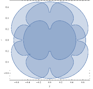
I've been playing around with some d-orbitals and have been trying to view their maximum in two dimensions. At the moment I've progressed to the point where the d__ orbitals are superimposed onto one another, in 2d, using a modification of Jens' answer here but have not managed to obtain the outline. Please pardon the code, its probably a bit convoluted and ever so slightly messy:

{rMin[n_, l_], rMax[n_, l_]} = r /. Simplify[Solve[(l (l + 1))/r^2 - 2/r == -(1/n^2), r], n > 0];

sphericalToCartesian = Thread[{r, θ, ϕ} -> {Sqrt[x^2 + y^2 + z^2], ArcCos[z/Sqrt[x^2 + y^2 + z^2]], Arg[x + I y]}];

(*The radial orbitals here are approximated using a Slater-type orbital using Clementi's atomic constants for Fe; see Slater-type orbitals on Wikipedia for further information*)
pimp[n_, l_, m_][r_, θ_, ϕ_] := (2*22.27)^n ((2*22.27)/(2 n)!) (r^(n - 1)) (E^(-22.27 r)) (Im[SphericalHarmonicY[l, m, θ, ϕ]] + Im[SphericalHarmonicY[l, -m, θ, ϕ]])
pimn[n_, l_, m_][r_, θ_, ϕ_] := (2*22.27)^n ((2*22.27)/(2 n)!) (r^(n - 1)) (E^(-22.27 r)) (Im[SphericalHarmonicY[l, m, θ, ϕ]] - Im[SphericalHarmonicY[l, -m, θ, ϕ]])
prep[n_, l_, m_][r_, θ_, ϕ_] := (2*22.27)^n ((2*22.27)/(2 n)!) (r^(n - 1)) (E^(-22.27 r)) (Re[SphericalHarmonicY[l, m, θ, ϕ]] + Re[SphericalHarmonicY[l, -m, θ, ϕ]])
pren[n_, l_, m_][r_, θ_, ϕ_] := (2*22.27)^n ((2*22.27)/(2 n)!) (r^(n - 1)) (E^(-22.27 r)) (Re[SphericalHarmonicY[l, m, θ, ϕ]] - Re[SphericalHarmonicY[l, -m, θ, ϕ]])

(*To get a 2d plot, I set the earlier evaluation so that x->0*)
plot2dx0[f_, range_, contour_, opt : OptionsPattern[]] := RegionPlot[Evaluate[Abs[f[r, θ, ϕ] /. sphericalToCartesian]^2 >contour] /. x -> 0, {y, -range, range}, {z, -range, range}]

(*Plotting the different d-orbitals*)
Show[plot2dx0[prep[3, 2, 0], 0.7, 0.00007], plot2dx0[pimp[3, 2, 1], 0.7, 0.00007], plot2dx0[pimn[3, 2, 2], 0.7, 0.00007], plot2dx0[pren[3, 2, 1], 0.7, 0.00007], plot2dx0[prep[3, 2, 2], 0.7, 0.00007], Frame -> True, FrameLabel -> {"y", "z"}]

(*Output*)

My question is then, whether it would be possible to (and how computational intensive would it be):

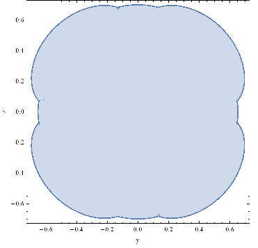
1. Obtain only the outline of this plot for visualisation so that the distance of this outline from the centre can be quantified (probably from pi to pi/2)
2. Plotting as a 2d density plot

For 1, it should look like:

For 1 & 2 I've tried the following which doesn't seem to work, and also summation of the terms (I've lost the code for that as the .nb didn't seem to save correctly on the train).

Evaluate[Max[{Abs[prep[3, 2, 0][1.12*r, θ, ϕ] /. sphericalToCartesian^2 > 0.0007],Abs[pimp[3, 2, 1][0.8*r, θ, ϕ] /. sphericalToCartesian^2 > 0.0007],Abs[pimn[3, 2, 2][1.12*r, θ, ϕ] /. sphericalToCartesian^2 > 0.0007],Abs[pren[3, 2, 1][1.12*r, θ, ϕ] /. sphericalToCartesian^2 > 0.0007],Abs[prep[3, 2, 2][1.12*r, θ, ϕ] /. sphericalToCartesian^2 > 0.0007]}]]

Could anyone please help/advise?

Many thanks, Z.