9
$\begingroup$

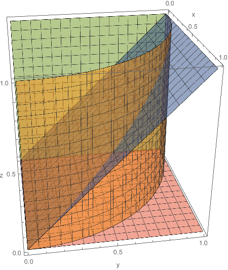
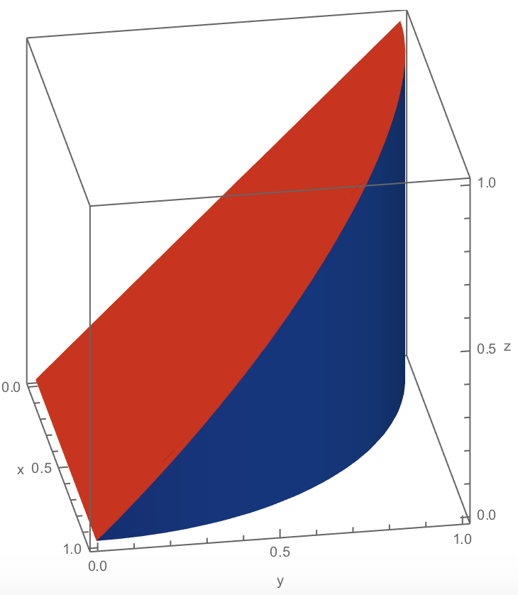
I need to draw (pencil and paper) the region bounded by $x^2+y^2=1$, $y=z$, $x=0$, and $z=0$ in the first octant. So the first assistance I asked of Mathematica is:

ContourPlot3D[{x^2 + y^2 == 1, y == z, x == 0, z == 0}, {x, 0, 1}, {y,
   0, 1}, {z, 0, 1},
 ContourStyle -> Opacity[0.5],
 AxesLabel -> {"x", "y", "z"},
 ViewPoint -> {3, -0.5, 1.5}]

Which gave me this image:

enter image description here

I was then able to draw the image via pencil and paper. Then I thought I'd try RegionFunction.

ContourPlot3D[{x^2 + y^2 == 1, y == z, x == 0, z == 0}, {x, 0, 1}, {y,
   0, 1}, {z, 0, 1},
 RegionFunction -> Function[{x, y, z}, y <= Sqrt[1 - x^2] && z <= y],
 ContourStyle -> Opacity[0.5],
 AxesLabel -> {"x", "y", "z"},
 ViewPoint -> {3, -0.5, 1.5}]

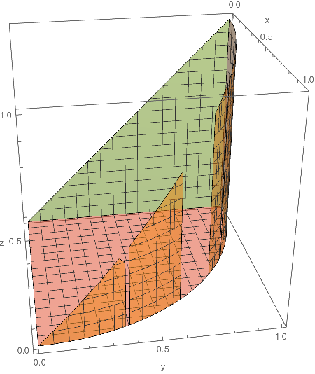
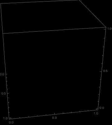
Which gave me this image.

enter image description here

I was able to repair it by extending my inequalities a bit.

ContourPlot3D[{x^2 + y^2 == 1, y == z, x == 0, z == 0}, {x, 0, 1}, {y,
   0, 1}, {z, 0, 1},
 RegionFunction -> 
  Function[{x, y, z}, y <= Sqrt[1 - x^2] + 0.001 && z <= y + 0.001],
 ContourStyle -> Opacity[0.5],
 AxesLabel -> {"x", "y", "z"},
 ViewPoint -> {3, -0.5, 1.5}]

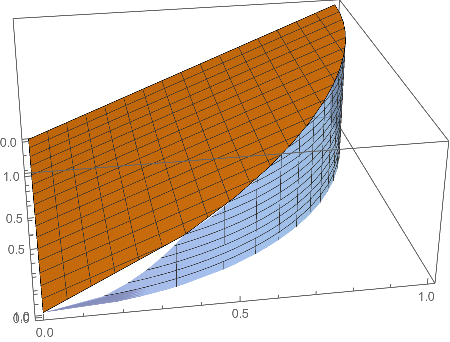
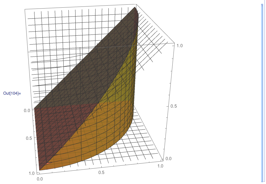
Which gave me this image.

enter image description here

Now, I am aware of RegionPlot3D, but I am not fond of the images it produces, although it is an easy method to get a quick idea of what the image looks like. So, I started trying a little ParametricPlot3D.

Show[
 Plot3D[y, {x, 0, 1}, {y, 0, Sqrt[1 - x^2]},
  AxesLabel -> {"x", "y", "z"}],
 ParametricPlot3D[{x, Sqrt[1 - x^2], z}, {x, 0, 1}, {z, 0, 
   Sqrt[1 - x^2]},
  PlotStyle -> {LightBlue, Opacity[0.8]}],
 ViewPoint -> {3, -0.5, 1.5}
 ]

Which gave me a little bit of strangeness. See the little sudden dipping in the border of the blue side as it approaches the x-axis?

enter image description here

I tried my contour inequality (adding 0.001 here an there) extension approach in several ways, but I could not get it to disappear. Any thoughts?

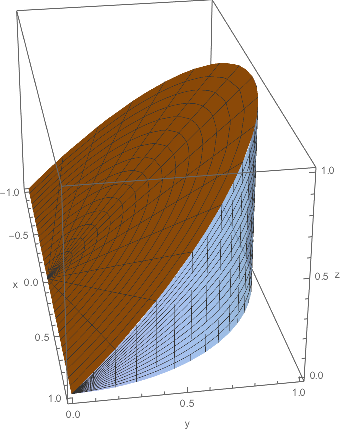
Update: There is some extremely wonderful work on this page, but I'd also like to add a cylindrical plot based on MichaelE2's suggestion.

Show[ParametricPlot3D[{u Cos[t], u Sin[t], u Sin[t]}, {t, 0, Pi}, {u, 
   0, 1},
  AxesLabel -> {"x", "y", "z"}], 
 ParametricPlot3D[{Cos[t], Sin[t], u Sin[t]}, {t, 0, Pi/2}, {u, 0, 1},
   PlotStyle -> {LightBlue, Opacity[0.8]}], 
 ViewPoint -> {3, -0.5, 1.5}]

enter image description here

$\endgroup$
3
  • 5
    $\begingroup$ Seen this? $\endgroup$ Commented Nov 2, 2015 at 5:57
  • 1
    $\begingroup$ Note one can do better in cylindrical coordinates and especially with direct construction of the surfaces. But judging from previous posts, I think the OP would prefer solutions that preserve the equations of the surfaces in cartesian coordinates -- Is that right, David? $\endgroup$
    – Michael E2
    Commented Nov 2, 2015 at 12:28
  • $\begingroup$ @MichaelE2 Yes, cylindrical would be OK. $\endgroup$
    – David
    Commented Nov 2, 2015 at 16:15

4 Answers 4

20
$\begingroup$

A simple alternative is to use Plot3D with both RegionFunction and Filling.

Plot3D[y, {x, 0, 1}, {y, 0, 1},
 RegionFunction ->
  Function[{x, y, z},
   x^2 + y^2 <= 1 && x >= 0 && y >= 0 && z >= 0],
 Filling -> 0,
 FillingStyle -> Opacity[.75],
 PlotStyle -> Opacity[.5],
 AxesLabel -> (Style[#, 14, Bold] & /@ {x, y, z}),
 BoxRatios -> {1, 1, 1},
 ViewPoint -> {3, -1.5, 0.75}]

enter image description here

EDIT: I recommend that you experiment with different settings for PlotTheme to determine which is best for your classroom and smartboard.

Manipulate[
 Plot3D[y, {x, 0, 1}, {y, 0, 1},
  RegionFunction -> 
   Function[{x, y, z}, 
    x^2 + y^2 <= 1 && x >= 0 && y >= 0 && z >= 0],
  Filling -> 0,
  FillingStyle -> Opacity[.75],
  PlotStyle -> Opacity[.5], 
  AxesLabel -> (Style[#, 18, Bold] & /@
     {x, y, z}),
  BoxRatios -> {1, 1, 1},
  ViewPoint -> {3, -1.5, 0.75},
  PlotTheme -> pt],
 {{pt, "Classic", "Plot Theme"},
  {"Business", "Classic", "Default",
   "Detailed", "Marketing", "Minimal",
   "Monochrome", "Scientific", "Web"}}]

enter image description here

$\endgroup$
2
  • $\begingroup$ Very nice, the easiest for the students to understand. I have another question. We use Smartboards in our classrooms to display our Mathematica images. What type of coloring in this example would make this image the easiest to see and interpret for students sitting in the back of the room and viewing the presentation on the Smartboard? $\endgroup$
    – David
    Commented Nov 2, 2015 at 16:18
  • $\begingroup$ Really nice going. I am going to give this a test today. $\endgroup$
    – David
    Commented Nov 2, 2015 at 21:06
8
$\begingroup$

As pointed out by J. M.♦, Simon Woods's approach in #48486 could be used.

sharpregplot[
  region_,
  {x_, x0_, x1_},
  {y_, y0_, y1_},
  {z_, z0_, z1_},
  opts : OptionsPattern[]
] := Module[
  {reg, preds},
  reg = LogicalExpand[region && x0 <= x <= x1 && y0 <= y <= y1 && z0 <= z <= z1];
  preds = Union@Cases[reg, _Greater | _GreaterEqual | _Less | _LessEqual, -1];
  Show @ Table[
    ContourPlot3D[
      Evaluate[Equal @@ p],
      {x, x0, x1},
      {y, y0, y1},
      {z, z0, z1},
      RegionFunction -> Function @@ {{x, y, z}, Refine[reg, p] && Refine[! reg, ! p]},
      opts
    ],
    {p, preds}
  ]
]

Then,

sharpregplot[
  y^2 <= 1 - x^2 && z <= y,
  {x, 0, 1}, {y, 0, 1}, {z, 0, 1},
  AxesLabel -> {"x", "y", "z"},
  BoundaryStyle -> None,
  ContourStyle -> RandomColor[],
  Mesh -> None,
  ViewPoint -> 1000 {3, -0.5, 1.5}
]

gives

Sharp RegionPlot3D

$\endgroup$
6
$\begingroup$

Here's one approach that uses MeshFunctions to highlight the parts of the bounding surfaces that belong to the region. So many different approaches are possible....

opts = Options[ParametricPlot3D];
SetOptions[ParametricPlot3D,
  {Mesh -> {{0}, 15, 15},
   MeshStyle -> Opacity[0.],      (* ignored -- bug? *)
   MeshShading -> {{{Automatic, None}}}}];
mfn["y==z"] = Function[{x, y, z, u, v}, z - y];
mfn["x^2+y^2==1"] = Function[{x, y, z, u, v}, x^2 + y^2 - 1];
Show[
 ParametricPlot3D[{x, y, y}, {x, 0, 1}, {y, 0, 1}, 
  PlotStyle -> {ColorData[97, 1], Opacity[0.8]},
  MeshFunctions -> {mfn["x^2+y^2==1"], #4 &, #5 &}],
 ParametricPlot3D[{x, Sqrt[1 - x^2], z}, {x, 0, 1}, {z, 0, 1}, 
  PlotStyle -> {ColorData[97, 2], Opacity[0.8]},
  MeshFunctions -> {mfn["y==z"], #4 &, #5 &}],
 ParametricPlot3D[{0, y, z}, {y, 0, 1}, {z, 0, 1}, 
  PlotStyle -> {ColorData[97, 3], Opacity[0.8]},
  MeshFunctions -> {mfn["y==z"], #4 &, #5 &}], 
 ParametricPlot3D[{x, y, 0}, {x, 0, 1}, {y, 0, 1}, 
  PlotStyle -> {ColorData[97, 4], Opacity[0.8]},
  MeshFunctions -> {mfn["x^2+y^2==1"], #4 &, #5 &}],
 ViewPoint -> {3, -0.5, 1.5}]
SetOptions[ParametricPlot3D, opts];

SE Uploader:

Hmm...it looks better on my screen (still a slight glitch in the corner):

enter image description here

Another bug? This often means Mathematica is about to crash. I think the OP has experienced this one before. (Note: I don't think this is a problem with the uploader. The same happens with Export and if I reevaluate the code. It's a hard to reproduce problem in the FE. I'm on Mac OSX V10.2)

$\endgroup$
4
$\begingroup$

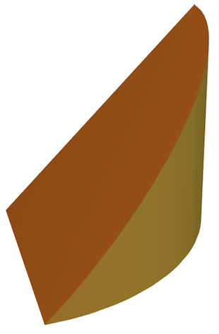
Just to cover more ways of achieving this. We can plot over a Disk and use a PlotTheme.

Plot3D[y, {x, y} ∈ Disk[{0, 0}, 1, {0, π/2}], PlotTheme -> "FilledSurface", 
  BoxRatios -> Automatic, Boxed -> False, Axes -> False]

enter image description here

$\endgroup$

Your Answer

By clicking “Post Your Answer”, you agree to our terms of service and acknowledge you have read our privacy policy.

Not the answer you're looking for? Browse other questions tagged or ask your own question.