Error NDSolve::nlnum1 from 2nd order ODE with 4 boundary conditions

Question

I want to solve this 2nd order ODE with two initial conditions close to the origin (one to the function and the other to its derivative) and more two similar conditions for an endpoint.

c = 0.5;
rzer = 0.001;
rmax = 10.000;
vmax = 0.550718236126181`;
dmax = -0.032852103365844154`;

shc0 = 
  NDSolve[
    {y''[r] + (1.` Csch[1.` r] - 1.25` Tanh[0.5` r]^2) y'[r] + 
      (-0.00048828125` Csch[0.5` r]^2 Sech[0.5` r]^4 
        (14.` + 139.` Cosh[1.` r] - 30.` Cosh[2.` r] + 5.` Cosh[3.` r] + 
          32.` Sinh[1.` r] - 16.` Sinh[2.` r])) y[r] == 0, 
     y[rzer] == rzer, y'[rzer] == rzer, y[rmax] == vmax, y'[rmax] == dmax},
    y[r], {r, rzer, rmax}]

But Mathematica 10 returns the message:

NDSolve::nlnum1 The function value {-0.001,-0.001,-0.550718,0.0328521} is not a list of numbers with dimensions {2} when the arguments are {0.,0.,0.,0.,0.,0.}.

My code only returns solutions when two values are fixed. Is there no way to solve this with the default method?

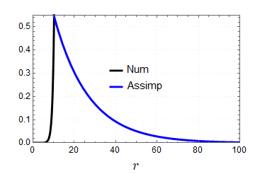
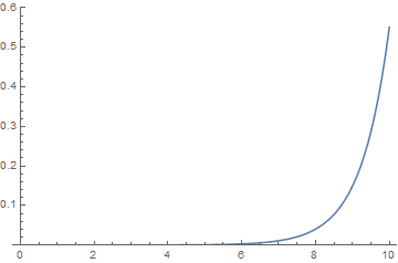
The aim of this problem was find a solution with these initial conditions (y'(0)=y(0)=0) that connects smoothly (preserves the slope) with an exponentially decreasing solution asymptotically, so have a finite integration in the interval with value greater that precision rzer (0.001).

I suppose that is not possible obtain a solution that satisfies all conditions imposed.

Thanks again.

Answer 1

The limit of two boundary conditions is not imposed by Mathematica. Rather, it is intrinsic to solving 2nd order ODEs. So, the number of boundary conditions must be reduced to two. Begin with the boundary condition at large r. According to the figure in the question, the solution should go asymptotically to zero there. The expression in the question, with numbers rationalized, is

eq = y''[r] + (Csch[ r] - 5/4 Tanh[r/2]^2) y'[r] + (-1/2048 Csch[r/2]^2 Sech[r/2]^4 
     (14 + 139 Cosh[r] - 30 Cosh[2 r] + 5 Cosh[3 r] + 32 Sinh[r] - 16 Sinh[2 r])) y[r];

With

rzer = 1/1000; rmax = 30;

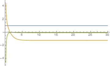
the coefficients in eq can be plotted as

Plot[Evaluate[Coefficient[eq, #] & /@ {y''[r], y'[r], y[r]}], {r, rzer, rmax}]

Because the coefficients become constant asymptotically, the ODE easily is solved for large r.

coef = Limit[Coefficient[eq, #], r -> Infinity] & /@ {y''[r], y'[r], y[r]}
(* {1, -(5/4), -(5/64)} *)
DSolve[coef.{y''[r], y'[r], y[r]} == 0, y[r], r]
(* {{y[r] -> E^((5/8 - Sqrt[15/2]/4) r) C[1] + E^((5/8 + Sqrt[15/2]/4) r) C[2]}} *)

Clearly, the exponentially decaying solution is desired.  Obtain its decay rate.

exp = Cases[%, Exp[z_] -> z/r, {0, Infinity}][[1]]
(* 5/8 - Sqrt[15/2]/4 *)

The boundary condition that fits the numerical solution at small r to the asymptotic solution is

y'[rmax] - exp y[rmax] == 0

Because the ODE is singular at the origin, a plausible boundary condition at rzer is that suggested by the OP

y[rzer] == rzer

With these boundary conditions,

s = First@NDSolve[{eq == 0, y[rzer] == rzer, y'[rmax] == exp y[rmax]}, 
    y, {r, rzer, rmax}, WorkingPrecision -> 45];
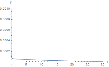
Plot[y[r] /. s, {r, rzer, rmax}, PlotRange -> All, AxesLabel -> {r, y}]

Addendum

Expanding the ODE at r == 0,

Series[eq, {r, 0, 1}] // Normal
(* - y[0]/(4*r^2) + (3*Derivative[1][y][0])/(4*r) + (y[0]/12 + 15*Derivative[2][y][0]/8) + 
  (r*(3*y[0] - 8*Derivative[1][y][0] + 140*Derivative[3][y][0]))/96 *)

shows that not only the ODE but also its solution is singular at the origin. For that reason, it might make more sense to use

vmax = Rationalize[0.550718236126181, 0];
y[10] = vmax 

as the second boundary condition. Then, with rmax increased to 50.

s = First@NDSolve[{eq == 0, y[10] == vmax, y'[rmax] - exp y[rmax] == 0}, 
    y, {r, rzer, rmax}, WorkingPrecision -> 55, MaxSteps -> 100000];
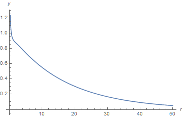
Plot[y[r] /. s, {r, rzer, rmax}, AxesLabel -> {r, y}]

This second solution is not better than the first in this answer, just rescaled. Note that further increasing rmax requires that WorkingPrecision also be increased, which makes the computation quite slow.

Answer 2

Trying using the following code. You can use three boundary values, but notice the same solution if you substitute the fourth boundary involving y'[rmax]=dmax. To this end, one of the boundaries is redundant.

c = 0.5; 
rzer = 0.001; 
rmax = 10.; 
vmax = 0.550718236126181; 
dmax = -0.032852103365844154; 
sols = 
   (First[
     NDSolve[{Derivative[2][y][
          r] + (1.*Csch[1.*r] - 1.25*Tanh[0.5*r]^2)*
          Derivative[1][y][
           r] + (-0.00048828125*Csch[0.5*r]^2*Sech[0.5*r]^4*
                       (14. + 139.*Cosh[1.*r] - 30.*Cosh[2.*r] + 
              5.*Cosh[3.*r] + 32.*Sinh[1.*r] - 16.*Sinh[2.*r]))*y[r] == 
        0, y[rzer] == rzer, y[rmax] == vmax}, y, r, 

      Method -> {"Shooting", 
        "StartingInitialConditions" -> {y[rzer] == rzer, 
          Derivative[1][y][rzer] == #1}}]] & ) /@ {rzer}

Plot the output using

Plot[Evaluate[y[r] /. sols], {r, rzer, rmax}, PlotRange -> {0, 0.6}]

With regard to your last answer, you can consider a second region r> 10, and then just use the last boundary condition. No need to employ the shooting method:

c = 0.5; rzer = 0.001; rmax = 10.; vmax = 0.550718236126181; dmax = \
-0.032852103365844154; 
  sols2 = 
 NDSolve[{Derivative[2][y][r] + (1.*Csch[1.*r] - 1.25*Tanh[0.5*r]^2)*
      Derivative[1][y][r] + 
            (-0.00048828125*Csch[0.5*r]^2*
        Sech[0.5*r]^4*(14. + 139.*Cosh[1.*r] - 30.*Cosh[2.*r] + 
          5.*Cosh[3.*r] + 32.*Sinh[1.*r] - 16.*Sinh[2.*r]))*y[r] == 0, 
        y[rmax] == vmax, Derivative[1][y][rmax] == dmax}, 
  y, {r, 10, 30}]

Notice that r > = 10