6
$\begingroup$

I would like to make an intensity plot of Bosons in a harmonic trapping potential. Hence, I would like to execute the following double summation (everything made dimensionless) for as many terms as possible

wavefunc[x_, n_] := 
1/(Sqrt[2^n Factorial[n] Sqrt[π]]) Exp[-x^2/2] HermiteH[n, x]

Intensity[x_, y_, μ_, nxmax_, nymax_] := Sum[(1/(Exp[((nx + ny + 1)/25 - μ)] - 1))
           (wavefunc[x, nx]* wavefunc[y, ny])^2, {nx, 0, nxmax}, {ny, 0, nymax}]

Subsequently I would like to plot as follows

Plot[Intensity[x, 0, -1/5, 75, 75], {x, -15, 15}].

Note that the factor of 1/25 in the intensity expression above is related to a certain value of the temperature. A typical value for $\mu$ would be $-1/5$. However, if I take $n_{x_{max}} = n_{y_{max}} = 75$, this already takes a very long time. I am aware that the number of terms goes as $O(n^2)$. Still, I would be very happy if there would be some way to speed this up in Mathematica by some option of some sort, as I only expect full convergence for $n_{x_{max}}$ a multiple of 25.

$\endgroup$
5
  • $\begingroup$ Note: you have missed the closing round bracket in wavefunc $\endgroup$
    – Hubble07
    Commented Sep 21, 2015 at 15:50
  • $\begingroup$ You can memoize wavefunc. That should make it way quicker. $\endgroup$ Commented Sep 21, 2015 at 15:58
  • $\begingroup$ The biggest problem probably is that Intensity is defined using SetDelayed, which forces Plot to evaluate the sum for every single choice of x value. Do instead With[{plt = Intensity[x, 0, -1/5, 75, 75]}, Plot[plt, {x, -15, 15}]]. $\endgroup$
    – march
    Commented Sep 21, 2015 at 16:07
  • $\begingroup$ @march I did have something like that before, but somehow Mathematica cannot handle the number of terms in the sum, which one can see by comparing the plots for nmax=60 and 75. There seem to be some divergences which are definitely not in the mathematical expression. $\endgroup$
    – Funzies
    Commented Sep 21, 2015 at 16:13
  • $\begingroup$ Sure, I saw those, too, and I assumed that there was some sort of numerical error occurring, but they seem to appear in your version as well. If you look at the expression that Intensity spits out, there are some HUGE numbers appearing. It's not wonder that there are numerical issues. Anyway, your question was about speed-up, which the With solution (or one of @MarcoB's solutions below) fixes. $\endgroup$
    – march
    Commented Sep 21, 2015 at 16:16

1 Answer 1

6
$\begingroup$

You can do two things: 1) use machine-precision evaluation, rather than arbitrary precision ones as you are currently doing; 2) memoize the wavefun function so values used more than once do not have to be recalculated.

intensity[x_, y_, μ_, nxmax_, nymax_] := Sum[(1/(Exp[((nx + ny + 1)/25 - μ)] - 1)) (wavefunc[x, nx]*wavefunc[y, ny])^2, {nx, 0, nxmax}, {ny, 0, nymax}]

(* original definition, for comparison *)
Clear[wavefunc]
wavefunc[x_, n_] := 1/(Sqrt[2^n Factorial[n] Sqrt[π]]) Exp[-x^2/2] HermiteH[n, x]
intensity[x, 0, -1/5, 75, 75]; // AbsoluteTiming

(* machine precision: note the 1. instead of 1 *)
Clear[wavefunc]
wavefunc[x_, n_] := 1./(Sqrt[2^n Factorial[n] Sqrt[π]]) Exp[-x^2/2] HermiteH[n, x]
intensity[x, 0, -1/5, 75, 75]; // AbsoluteTiming

(* memoized and machine-precision *)
Clear[wavefunc]
wavefunc[x_, n_] := wavefunc[x, n] = 1./(Sqrt[2^n Factorial[n] Sqrt[π]]) Exp[-x^2/2] HermiteH[n, x]
intensity[x, 0, -1/5, 75, 75]; // AbsoluteTiming

Timing results are as follows:

original:                       3.96246 s
machine-precision evaluation:   1.29093 s ( 3x faster)
machine precision and memoized: 0.11249 s (36x faster)

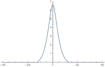
UPDATE: As you and @march mentioned, your expressions suffer from numerical precision issues probably due to the Hermite polynomials. Machine-precision evaluation is therefore inadvisable, but still, combining memoization of arbitrary-precision wavefun with calculating intensity only once before passing it to Plot should give an appreciable speedup.

Clear[wavefunc]
wavefunc[x_, n_] :=
  wavefunc[x, n] =
   1/(Sqrt[2^n Factorial[n] Sqrt[\[Pi]]]) Exp[-x^2/2] HermiteH[n, x]

(plot = With[
     {expr = intensity[x, 0, -1/5, 75, 75]},
     Plot[expr, {x, -40, 40}, PlotRange -> All, WorkingPrecision -> 20]
   ];) // AbsoluteTiming

plot

(* Out: {13.9598, Null} *)

plot

$\endgroup$
3
  • $\begingroup$ Note the most recent comment by the OP in the OP. There are also some numerical stability issues it seems. $\endgroup$
    – march
    Commented Sep 21, 2015 at 16:17
  • $\begingroup$ @march I noticed that as well, while playing with the machine-precision version. I amended my answer accordingly, also including your suggestion to prevent needless recalculation of the intensity expression. $\endgroup$
    – MarcoB
    Commented Sep 21, 2015 at 16:27
  • 1
    $\begingroup$ @MarcoB Thanks for your reply. Indeed, your code gives a good speed-up. However, to ensure convergence I need to take a lot more terms into account. Going to 100 terms, the results becomes 'weird', probably due to numerical errors as you mentioned. Is there any way this can be fixed? $\endgroup$
    – Funzies
    Commented Sep 22, 2015 at 9:22

Your Answer

By clicking “Post Your Answer”, you agree to our terms of service and acknowledge you have read our privacy policy.

Not the answer you're looking for? Browse other questions tagged or ask your own question.