Sorry in advance for my logorrhea: I just want to make sure all of the information is here.
Context and Question
I am investigating site percolation on a square lattice. I have a working, depth-first, recursive clustering algorithm. The algorithm as coded is recursive but procedural, so I want to find a way to mimic the recursive nature of the algorithm using Mathematica's functional-programming style. In addition, the Kernel dies if the number $l^2$ of grid points is too large and if the filling fraction is large enough that the percolating cluster is very large; I presume this is due to the large recursion depth of the search. (If coded in C, I can do much larger lattice sizes and filling fractions.) Therefore, I would like a way of getting around this problem of the Kernel crashing. In summary, I would like to:
Mimic the recursive algorithm with functional-programming.
Get around the problem of the
Kernelcrashing due to the large recursion depth of the algorithm (presumably this is solved by fulfilling the previous bullet point).
I have tried to come up with a way of implementing this using functions like Nest or Fold, but I can't see how to mimic the tree-nature of the recursive search, since they seem not to be able to deal with trees.
One last point: this algorithm is fast (EDIT: apparently, no, it's not: see Update below). It may be that implementing a functional programming version in Mathematica will be slower. In that case, I am still interested in the answer for the purpose of honing my functional programming skills.
Algorithm Description
The input is an $l\times l$ array configuration consisting of $-1$'s at filled sites and $0$'s elsewhere. The output consists of a list of {clusterNumber,clusterSize}s and an $l\times l$ array with the $-1$'s replaced by the corresponding cluster number and the $0$'s left alone. Sites belong to the same cluster if they are nearest neighbors (diagonals not allowed). As an example in a $4\times4$ lattice,
inputConfiguration={{-1,-1,-1,0},{-1,0,0,-1},{-1,-1,0,-1},{0,-1,0,0}};
output={{1,7} , {2,2} , {{1,1,1,0},{1,0,0,2},{1,1,0,2},{0,1,0,0}}};
Below, you will see that the configurations are Flattened. This is merely a programming convenience. To go from one version to another, I either Flatten[configuration] or Partition[configuration,l].
Before talking about the algorithm specifically, note that
neighbors[l_]= DeleteCases[{If[-l + # >= 0, -l + #, -1],
 If[Quotient[-1 + #, l] == Quotient[#, l], -1 + #, -1],
 If[Quotient[1 + #, l] == Quotient[#, l], 1 + #, -1],
 If[l + # <= l^2 - 1, l + #, -1]} + 1, 0] & /@ Range[0, l^2 - 1]
is a function that returns a list of the indices of the neighboring sites of each site, where the indices correspond to the flattened configuration. For instance,
neighbors[4][[2]] = {1,3,6}
because site number 2 is bordered by site 1 on the left, 3 on the right, and 6 below. (This can certainly be implemented in a nicer way, so feel free to fix this, but this is not the focus of this question.)
The heart of the algorithm is the recursive function cluster that accepts the current site index i and cluster number clusterNumber as inputs, sets the current grid value to clusterNumber, then checks the neighbors of site i. If a neighbor site j is a filled site but has not yet been assigned a cluster number, cluster is called with inputs j and clusterNumber. A function call to cluster will terminate once the input site j has no neighbors not yet part of a cluster, and once all recursive calls to cluster have terminated, all sites in the current cluster have been labeled with clusterNumber.
At this point, I Sow both the current cluster number and the current cluster size and then move on. At the end, I Sow the clustered configuration.
Code
In practice, I run the code in a Block in order to set the $RecursionLimit larger, which is necessary for larger lattice sizes and larger filling fractions. For instance, for the $4\times4$ configuration above, we would call the function as
Block[{$RecursionLimit=10000}, Reap[clustering[inputConfiguration, neighbors[4],4]]]
Here is the code:
clustering[configuration_, boundaries_, l_] := Module[{
  grid = Flatten[configuration]
  ,cluster
  ,clusterNumber = 1
  ,clusterSize
 }
 ,cluster[i_, num_] := Module[{}
    ,grid[[i]] = num
    ;clusterSize = clusterSize + 1
    ;If[grid[[#]] < 0, cluster[#, num]] & /@ boundaries[[i]]
   ]
 ;Do[
   If[grid[[m]] < 0
    ,clusterSize = 0
    ;cluster[m, clusterNumber]
    ;Sow[{clusterNumber++, clusterSize}]
   ]
   , {m, 1, l^2}]
   ;Sow[Partition[grid,l]]
  ]
 ]
Further Goals
It is also useful to return a list of {clusterNumber,clusterIndices}s, where clusterIndices is a list of the site indices of the cluster labeled clusterNumber. Presumably, given code that mimics the code above with functional programming, I would be able to modify it in order to return the clusterIndices rather than the clusterSize, so this is not a top priority, but perhaps it's important to keep in mind.
Update: Benchmarking the cluster algorithms
I have stripped out the clusterSize and clusterIndex finding from the original code and Virgil's two versions (the image-processing version and the recursive version) in order to benchmark just the clustering algorithms.
Specifically, I have a random configuration function that randomly chooses site indices to fill and returns the grid in the correct format:
randomConfiguration[l_, nf] := Block[
  {grid = ConstantArray[0, l^2], config = RandomSample[Range[l^2], nf]}
  , grid[[config]] = -1; Partition[grid,l]]
I have then defined the three clustering codes. First, the original, essentially:
march[config_] := Module[{grid = Flatten[config], l = Length@config, clusterSearch, num = 1, boundaries}
  , boundaries = DeleteCases[{If[-l + # >= 0, -l + #, -1],
      If[Quotient[-1 + #, l] == Quotient[#, l], -1 + #, -1],
      If[Quotient[1 + #, l] == Quotient[#, l], 1 + #, -1],
      If[l + # <= l^2 - 1, l + #, -1]} + 1, 0] & /@ Range[0, l^2 - 1]
  ; clusterSearch[i_, num_] := Module[{}
      , grid[[i]] = num
      ; If[grid[[#]] < 0, clusterSearch[#, num]] & /@ boundaries[[i]]
    ]
  ; Do[If[grid[[m]] < 0 , clusterSearch[m, num] ; num++ ] , {m, 1, l^2}]
  ; Partition[grid, l]
]
Then, Virgil's recursive code:
virgilRec[config_] := Module[{output = config, cnum = 0, length = Length@config, csearch}
  , csearch[{i_, j_}, cnum_] := If[output[[i, j]] == -1
      , output[[i, j]] = cnum
      ; csearch[#, cnum] & /@ Select[{i, j} + # & /@ {{0, 1}, {0, -1}, {1, 0}, {-1, 0}}, (1 <= First@# <= length && 1 <= Last@# <= length) &]
    ]
  ; Scan[
      If[output[[Sequence @@ #]] == -1
        , cnum++
        ; csearch[#, cnum]
      ] &
      , SparseArray[config]["NonzeroPositions"]
    ];
  output];
Finally, Virgil's image-processing code:
virgilImage[config_] := Module[{output, csizes, cindices}
  , output = MorphologicalComponents[Image@Abs@config, CornerNeighbors -> False]
  ; output];
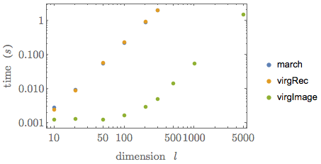
For each, I chose 50 random configurations at a filling fraction of $\approx0.593$ for various choices of $l$ and averaged the times taken to complete the clustering process, using
benchmark[f_, l, frac_] := With[{config = randomConfiguration[l,frac]}
  , {l, Mean@Table[First@AbsoluteTiming@f@config, {50}]}
  ]
The results are interesting!

In both recursive codes, the clustering time grows as a power law with the grid dimension from the beginning, whereas in the image processing version, the time is flat for a good while. Eventually, the clustering time in virgilImage grows as a power law as well. The slopes of the linear regions of the plots are all basically 2, which indicates that the clustering time grows linearly with the number $l^2$ of grid points for large enough $l$. virgilImage is a clear winner from the get-go.
To do
- Per a comment, see whether
virgilImageis faster if we don't convert the grid to an image first. - See if we can implement
SparseArrayas a convenient data structure for the grid. - Take advantage of the fact that in choosing the random configuration, we have the indices of the filled sites from the beginning, which means we can combine the grid "data structure" with the list of filled site indices in order not to have to call the
NonzeroPositionsMethod. - Wait for more answers (hopefully)! I am still interested in seeing the experts' take on Mathematica-style recursive algorithms.

