This is a classic example from documentation center. I will modify this slightly, to make it more complex.
A = RandomReal[{0, 1}, {5, 5}];
Now you can actually mix scalar and vector functions - 'NDSolve' will understand it:
fs = x /.First[NDSolve[{x'[t] == 1 - Norm[x[t]] A.Sin[x[t]],
      x[0] == RandomReal[1, 5]}, x, {t, 0, 23}]];
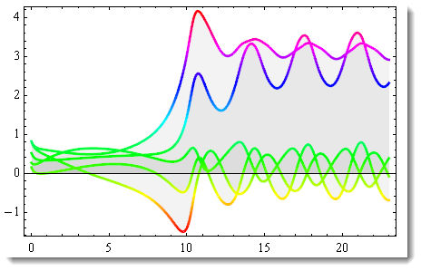
Visualize typically:
Plot[fs[t], {t, 0, 23}, ColorFunction -> Hue, PlotStyle -> Thick,
 Frame -> True, FillingStyle -> Opacity[0.05], Filling -> 0]

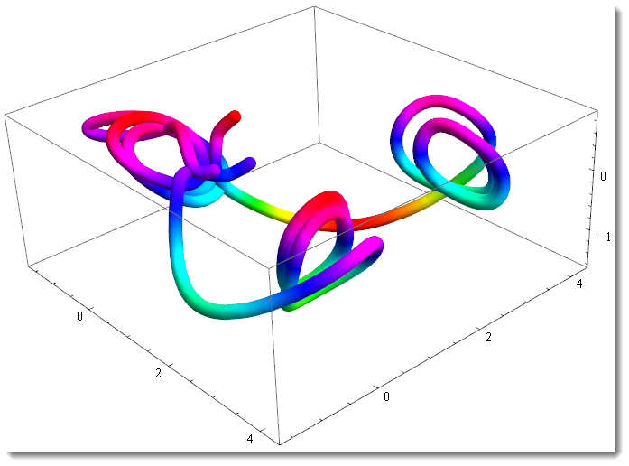
Or visualize in an interesting way:
ParametricPlot3D[ fs[t][[#1 ;; #2]] & @@@ {{1, 3}, {2, 4}, {3, 5}}, {t, 0, 23},
  PlotRange -> All, PlotStyle -> Thick, ColorFunction -> Hue,
  ImageSize -> 450] /. Line[pts_, rest___] :> Tube[pts, 0.1, rest]


rhs. The added ingredient here is to useArrayto generate the vectors. $\endgroup$rhs[Y[t]]does not have a symbolic form. That is what I meant by "numerically calculates". $\endgroup$