11
$\begingroup$

I'm trying to find the determinant of a band diagonal matrix that has a parameter, $\kappa$, in some of the entries. Some entries are just numerical ones, others ($\kappa$ X number), while others are ($\kappa$ + number). I have been told that they way to solve for $\kappa$ is to find the determinant of the this matrix and then find values of $\kappa$ that make the determinant zero.

The main issue I'm having is that when my matrix becomes large the determinant just results to zero,and in other cases to calculation overflow. (I'm trying to work out all the bugs in the code, so det =0, might be some error I'm making, but the overflow error is not avoidable).

I have already tried an LUDecomposition on the matrix, and that seems to take forever, I don't have a problem waiting, but working out the scaling, it seemed like I would have to wait a couple of days for a 500X500 matrix, and my real problem might have to be done on a 1000X1000 matrix.

I was also thinking that maybe I could somehow get the matrix into an upper triangular form and then just multiply the diagonal elements. For this I tried using Mathematica's RowReduce command, but for some weird reason that just results in the identity matrix. I thought that RowReduce might give me an upper triangular matrix with $f(\kappa)$ on the diagonal, and I could just multiply the diagonal elements and get a polynomial for $\kappa$ and solve.

Any and all help is greatly appreciated. I'm not really sure how to put up my code, or the matrix for that matter. That is the thing that would probably help you guys the most. If there is a way for me to put up the matrix please let me know.

Thanks again.

EDIT- A matrix that gives you guys some idea of my matrix.

t2 = {{-892.33, 973.21, 44.306 + \[Kappa], -81.103,0}, 
 {446.12, -557.94, 0, -682.54, -314.89}, 
 {0,893.37, -506.68*\ [Kappa],-391.457, 0}, {0, 429.78, 0, -210.47, 
 342.85}, {278.32*\[Kappa], 0, 963.41, 217.71, -342.68 + \[Kappa]}} 

2nd-EDIT Although I do not fully understand what Jens' code is doing I did try it on my real matrix. The result is

In[193]:= f[\[Kappa]_?NumericQ] := 
 Min[Diagonal[SingularValueDecomposition[mat][[2]]]]
In[194]:= Plot[f[\[Kappa]], {\[Kappa], 0, 2}]

Well being a noob the site won't let me upload an image, but it basically looks like there should be roots around $\kappa$ = .1, .2, .4,.4, .6.

So I tried to find the root using

In[196]:= FindRoot[f[x], {x, .5}]

And then I get a bunch of error messages.

During evaluation of In[196]:= InterpolatingFunction::dmval:
Input value {-0.173686} lies outside the range of data 
in the interpolating function.Extrapolation will be used. >>

During evaluation of In[196]:= InterpolatingFunction::dmval: 
Input value {-0.173686} lies outside the range of data in the 
interpolating function. Extrapolation will be used. >>

During evaluation of In[196]:= InterpolatingFunction::dmval: 
Input value {-0.173686} lies outside the range of data 
in the interpolating function. Extrapolation will be used. >>

 During evaluation of In[196]:= General::stop: Further output of   
 InterpolatingFunction::dmval will be suppressed during this calculation. >>

 Out[196]= {x -> -3.28829*10^-13}

So I figured that if root-finder couldn't do it, I'd just try it by hand, i.e. just look at the plot and keep narrowing down the point where f($\kappa$) =0, so I tried to evaluate

 In[190]:= f[.2]

which was taking forever considering that this command

In[193]:= f[\[Kappa]_?NumericQ] := 
Min[Diagonal[SingularValueDecomposition[mat][[2]]]]

and the plot command both took less than an second. I'm very confused.

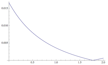
3rd Edit I think I can post a picture now. So I will include my plot for f[x]. This might make it easier to figure out what is going wrong with root-finder. I'm thinking its the multiple roots.
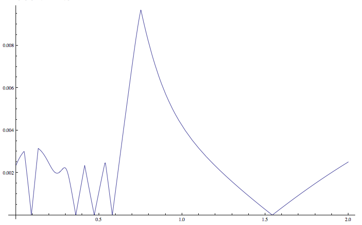
enter image description here

4th Edit Hi All, Happy almost 4th of July,

There is some good news and some bad news about the code thus far. The good news is that it seems to be working fine for larger grid sizes. I haven't cranked it up too much b/c my computer can't really handle it. The bad news is that I'm getting complex solutions. I know that the physical problem I am dealing with should not have complex solutions. Therefore when I was implementing the code by finding det(mat($\kappa$)= 0 , and solving the resulting polynomial for the roots I was using Solve[d1 == \[Kappa], Reals], where d1 = Det[mat]. This allowed me to only examine the real roots. However using the code

g[x_?NumericQ] := Last[SingularValueList[mat /. \[Kappa] -> x]]
Plot[g[x], {x, .5, 2/3}]

Gives me the following plot
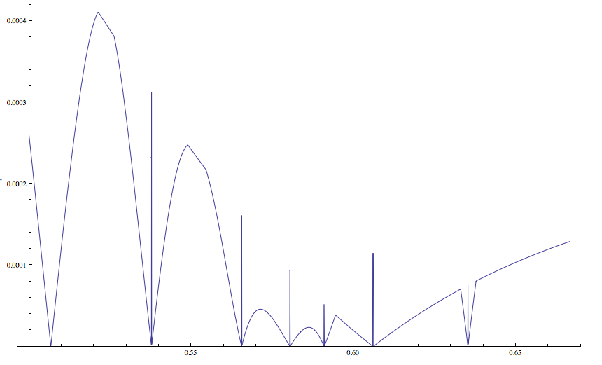
SVD-updatedPlot

and then I try FindRoot[g[x], {x, .58, .55, .6}]. Which results in {x -> 0.580341}, and the following error message

FindRoot::lstol: The line search decreased the step size to within tolerance    
specified by AccuracyGoal and PrecisionGoal but was unable to find a 
sufficient decrease in the merit function. You may need more than 
MachinePrecision digits of working precision to meet these tolerances. >>

Which I looked up and is supposed to mean that root finder cannot find real roots. So my first question is: what does {x -> 0.506739}, mean if Mathematica couldn't find real roots?

I've also tried to increase the AccracyGoal and WorkingPresicion with this

FindRoot[g[x], {x, .58, .55, .6}, AccuracyGoal -> MachinePrecision,     
WorkingPrecision -> 20]

Which results in a similar error.

FindRoot::lstol: The line search decreased the step size to within tolerance 
specified by AccuracyGoal and PrecisionGoal but was unable to find a 
sufficient decrease in the merit function. You may need more than 20.` 
digits of working precision to meet these tolerances. >>

So I'm quite lost as to where to go now. I've gone through my code and made sure that I put everything in fractional form, i.e. 1/2 instead of .5 since I know that can reduce precision, and make Mathematica angry.

As an aside, I wanted to throw another question out there. From the plot we can see that there are many roots present. And that there will be even more when I make the grid-size larger. I've already restricted the values for $\kappa$ to what is physically possible (in the Plot command), but that stills results in 10 -20 roots. Is there any other way to know which root is the real physics answer?

5th Edit New plot with Jens' suggestion used in code.
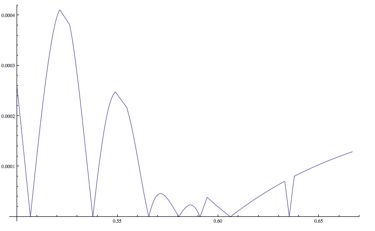
SVD-plot3

Now there are also no errors when I try the FindRoot command.

6th Edit,So this strange...or is it? If I understand the procedure that we have worked out thus far, the plots that I created above tell me "how singular" my matrix is as a function of my parameter $\kappa$. Thus I would probably like my y-axis to be really small, and so I am telling SingularValueList to only give me the last entry since that should be the smallest singular value, and also why I'm using the tolerance function,so that the smallest value do not get ignored. One question is, why use tolerance if were are already looking at the smallest singular value? The other problem, the strange part, is that when I find a $\kappa$ using SVL, and root finding command, then write $\kappa = .508...$, and then Det[mat], I get something like 2.14^113, and 1.678^109, for another root. Is that right? Is this essentially as close to zero as we can get the determinant? Or am I missing something huge. Is it that I am using the wrong root. Is there one that can give me Det = .0000001 or even smaller? I guess its not all bad news, this smalleness of the Det could help me figure out which is the true root. Anyways just throwing some thoughts/questions out there. Thanks again to all who respond. This problem is starting to drive me crazy but I guess that research.

$\endgroup$
12
  • $\begingroup$ Should it be FindRoot[f[\[Kappa]],{\[Kappa],.5}]? There was an x. Could this have generated the error messages? $\endgroup$
    – night owl
    Commented Jun 28, 2012 at 6:43
  • $\begingroup$ @nightowl, I just checked with $\kappa$ instead of "x" it did not make a difference. I didn't think it would since I defined the function "f" it should have been able to take any variable as it input. Thanks for help, at least that part is troubleshot. $\endgroup$
    – tau1777
    Commented Jun 28, 2012 at 7:01
  • $\begingroup$ Are you sure kappa has finite roots? Plot[Det[t2], {\[Kappa], -10, 10}, AxesOrigin -> {0, 0}] (or Solve[Det[t2] == 0, \[Kappa]]) $\endgroup$
    – user1066
    Commented Jun 28, 2012 at 7:32
  • $\begingroup$ Finding the determinant of a symbolic matrix is very, very slow, and it gets bad fast. On my machine, I cap out at $11\times 11$ matrices (which take 4 secs) before Mathematica begins to chew up a lot of memory. Since you have a numerical matrix, $M$ plus a symbolic matrix of a single variable, $\kappa A$, it may be worthwhile to see if you can recast $A$ as a rank-1 or rank-l ($l\le n$) update. Then you can use the matrix determinant lemma. As this is non-trivial, I opted to just comment instead of providing an answer. $\endgroup$
    – rcollyer
    Commented Jun 28, 2012 at 16:45
  • $\begingroup$ @rcollyer Thanks for the suggestion. I'm not sure if I can rewrite my problem like this, since there are terms like $\kappa$a(1,1) etc, but this is certainly something I will look into. $\endgroup$
    – tau1777
    Commented Jun 28, 2012 at 16:50

2 Answers 2

10
$\begingroup$

Not knowing anything else about the matrix, I can only suggest another alternative to the determinant (which sounds like it's prohibitively time-consuming).

If m is your matrix, try to find a root (or minimum) of

Min@Diagonal@SingularValueDecomposition[m][[2]]

instead. Unfortunately, SingularValueDecomposition is also very time consuming, but as I said, I don't know your matrix and therefore you may be lucky and it works. The lowest singular value will become zero when the matrix is singular.

Simplification: The second part [[2]] of SingularValueDecomposition is a square diagonal matrix, and by applying Diagonal to it I extract the one-dimensional list of singular values. This isn't really necessary since we don't need the other parts of SingularValueDecomposition. If all you want is the list of singular values, you should use

Last@SingularValueList[m]

Edit

No matter what method you end up choosing to test for the singularity of the matrix, you should probably not do it symbolically. That is, you have to define a "merit" function with your parameter $\kappa$ as a numerical variable:

Here is a crude example of a matrix and the corresponding function f:

m = {{0.7407182168539275`, 0.24672805625057825`, 
   0.8493016773864293`}, {0.06662628477504584`, 0.3469746999275358`, 
   0.2741493334768361`}, {0.07058419213858214`, 0.9556414582722623`, 
   0.7252123775090984`}};

f[κ_?NumericQ] := 
 Last[SingularValueList[m + DiagonalMatrix[{κ, 0, 0}]]]

Edit 2: Explanation

The pattern f[κ_?NumericQ] insures that the function will return a value only if it is called with a numerical argument κ. Any minimization or root finding routine will by default attempt to simplify f[κ] symbolically, but since f is defined only for numerical arguments that attempt will fail. This is good because the automatic evaluator then chooses a purely numerical method, which in our case is faster.

The SetDelayed := in the function definition means that the evaluation on the right-hand side (i.e., the singular-value decomposition or any other decomposition you may choose) will only be performed at the time when the function is called with a numerical parameter κ. At that point, if everything else in the matrix is numerical, the entire matrix is a numerical matrix and the result will not involve anything symbolic.

Finally, the reason I take only the Last part of the SingularValueList is that it is automatically the smallest. The smallest singular value is the one that first hits zero when a matrix becomes singular. That it the point of zero determinant we're looking for.

There are complications when you work with matrices that are already close to being numerically singular, because in that case you'll have to decide how close to singular you want the matrix to get as you vary the parameter. In those cases one may have to look at the next higher singular values.

Here I plot the example f, which is now an "indicator" of how singular the matrix is:

Plot[f[κ], {κ, 0, 2}]

root

FindRoot[f[x], {x, 1}]

(* ==> {x -> 1.78179} *)

Applying this to your example:

f[κ_?NumericQ] := 
 Last[
   SingularValueList[{{-892.33`, 973.21`, 
       44.306` + κ, -81.103`, 0}, {446.12`, -557.94`, 
       0, -682.54`, -314.89`}, {0, 
       893.37`, -506.68` κ, -391.457`, 0}, {0, 429.78`, 
       0, -210.47`, 342.85`}, {278.32` κ, 0, 963.41`, 
       217.71`, -342.68` + κ}}]]

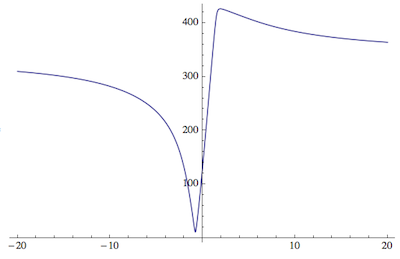
We can make a plot and realize that there won't likely be a zero for real values κ, but in the complex plane things look more promising:

Plot[Abs[f[κ - 2 I]], {κ, -20, 20}]

complex

Here I've subtracted an imaginary part from the real κ, and the curve seems to dip sharply down to close to zero. So let's try the following minimization:

sol = FindMinimum[Abs[f[x + I y]], {{x, -1}, {y, -2}}]

FindMinimum::lstol: The line search decreased the step size...

{1.89011*10^-6, {x -> -0.777723, y -> -2.07495}}

So there's still some work to do to get rid of the warning message, but in principle we got somewhere.

Edit 3

In order to make a pre-existing matrix mat (containing a parameter κ) into a function that you can use for root finding etc., you have to watch out for the difference between the global variable κ and the pattern instance κ that is passed to the function in place of the "dummy variable" in the pattern f[κ_?NumericQ].

The dummy variable could have equally well been named x_ or b_, so how do we make sure that it gets substituted into the matrix wherever the global variable κ appears?

Here is a way to do that. Assume the matrix is externally given as

Clear[κ]; mat = {{-892.33`, 973.21`, 44.306` + κ, -81.103`, 
    0}, {446.12`, -557.94`, 0, -682.54`, -314.89`}, {0, 
    893.37`, -506.68` κ, -391.457`, 0}, {0, 429.78`, 
    0, -210.47`, 342.85`}, {278.32` κ, 0, 963.41`, 
    217.71`, -342.68` + κ}};

Then change your function definition to

f[x_?NumericQ] := Last[SingularValueList[mat /. κ -> x]]

What this does is to replace the global κ (which you must make sure is unassigned, hence the Clear for safety) by the value of the dummy variable in the function. I have to change its name to something other than κ, so I chose x.

Edit 4

To capture what I said in some additional comments: if you do decide to use the lowest singular value as a merit function for further root finding or minimization, as a function of the parameter κ, then you may run into the problem that SingularValueList will omit the lowest singular values if they are too small relative to the largest singular value. This can lead to jumps if you plot the lowest singular value versus κ, because you aren't tracking the same singular value at all times. To insure that no singular values are omitted, one has to use

SingularValueList[m, Tolerance -> 0]

I can't answer the question of whether this is physically the best procedure, because I don't know what the physical problem is.

A very good mathematical discussion of the singular value decomposition is in Numerical Recipes in C on page 59.

$\endgroup$
14
  • $\begingroup$ Hi Jens, Thank you so much for the your response. I will definitely have to take a look at into the singular value decomposition idea. I think I follow most of what you did, but I'm not sure if I can apply this to my matrix. I should have done this earlier, but I created a fake matrix (I added it under my original post), which I believe gives a clearer idea of what I am dealing with. I'm not really sure I could use this SVDecomp trick with that matrix. Sorry to be a bother but could you please provide further instruction. You've hit upon the main issue, getting around doing it symbolically. $\endgroup$
    – tau1777
    Commented Jun 28, 2012 at 3:06
  • $\begingroup$ OK, so I actually understand [Diagonal[ SingularValueDecomposition[ m + DiagonalMatrix[{κ, 0, 0}]][[2]]]] that part of your code. You are creating a matrix with ($\kappa$ + number) at the (1,1) entry, and then preforming a SVD on that matrix. The [[2]]] allows you to call the second part of the SVD output, and Diagonal asks for the diagonal elements of the matrix that has all of the singular values. But I am still confused about f[κ_?NumericQ] := Min[. What does calling Min do? Also, I've never seen a function defined like this f[κ_?NumericQ] :=. Thanks again. $\endgroup$
    – tau1777
    Commented Jun 28, 2012 at 3:35
  • $\begingroup$ I've tried to add some more discussion - hope this helps with your actual matrix... $\endgroup$
    – Jens
    Commented Jun 28, 2012 at 5:05
  • $\begingroup$ Thank you very much Jens, I did not expect this much detail, you are wonderful. I need sometime to figure out why the Min or Last command needs to be called. And I also need to figure out why this technique seems to be failing in my real problem (details in my 2nd edit) , but I do very much appreciate the help. $\endgroup$
    – tau1777
    Commented Jun 28, 2012 at 5:37
  • $\begingroup$ I forgot to ask one important thing, and that is about the SVD. It seems to be that SVD returns something symbolic, and then only by creating a function that accepts numerically inputs are we making that numeric "merit function" you mentioned. Am I getting that right? The way I see it is that by plotting[f[x]]from 0 to 2, we are letting f[x] take numbers from 0 to 2 as numeric input and then it creates the plot you showed. I guess the crux of my question is that if SVD is symbolic then what is the real gain in using this than just doing Det[matrix]? $\endgroup$
    – tau1777
    Commented Jun 28, 2012 at 6:46
6
$\begingroup$

You can compute the determinant by interpolation, as below.

In[149]:= 
t2 = {{-892.33, 973.21, 44.306 + kappa, -81.103, 0}, {446.12, -557.94,
     0, -682.54, -314.89}, {0, 893.37, -506.68*kappa, -391.457, 
    0}, {0, 429.78, 0, -210.47, 342.85}, {278.32*kappa, 0, 963.41, 
    217.71, -342.68 + kappa}};

In[151]:= vals = Table[Det[t2], {kappa, 1, Length[t2] + 1}];

In[153]:= InterpolatingPolynomial[vals, kappa] // Expand

Out[153]= -2.05175*10^14 - 6.49939*10^13 kappa - 
 4.17848*10^13 kappa^2 + 1.8125 kappa^3 - 0.273438 kappa^4 + 
 0.015625 kappa^5

A big problem is that you are very likely to run into issues with numeric stability. If, as Jens suggests, you are trying to find a value of kappa for which the matrix becomes singular, his SVD approach looks to be more viable than working with the determinant.

$\endgroup$
5
  • $\begingroup$ Hi, Thank you so much for your response and for providing code. If I understand you're method you are calculating the determinant for values of $\kappa$ ranging form 1 to (length of the matrix+1). What is the reasoning for picking these bounds? I was planning on trying something like this myself, and now I have the code for it, thanks again. I don't know a lot about numeric stability, so I'm not quite sure what kind of problems to expect there. I'm sure these are problems I would like to avoid, but using SVD does take a while since things are still being done symbolically. Thanks. $\endgroup$
    – tau1777
    Commented Jun 28, 2012 at 17:00
  • $\begingroup$ Since kappa only appears linearly in the amtrix, we know the det is a polynomial in kappa of degree at most the dimension of the matrix. That accounts for the number of values I used. As for what values to pick, probably it would be numerically better to center them around the origin. But I doubt anything will be sufficient to gain numerically a nice expression, e.g. something you could extract accurate roots from (let alone take home to meet your parents). I think for the SVD you want to only compute it when kappa is given actual numeric values. Jens used this in his FindMinimum method. $\endgroup$ Commented Jun 28, 2012 at 17:12
  • $\begingroup$ Thanks for the reply. Indeed Jens' method would have been perfect, the main issue I'm running into that is that the root finder is failing. Also, I don't get the idea that SVD only computes when numerical values are passed to it. Doesn't mathematica first have to create a symbolic function from SVD using the input matrix with its $\kappa$ entries? There is something that I'm definitely missing since f[κ_?NumericQ] := Last[SingularValueList[m + DiagonalMatrix[{κ, 0, 0}]]] runs in 1 sec, but f[.2] or SVD[matrix],seems to take forever. Thanks again. $\endgroup$
    – tau1777
    Commented Jun 28, 2012 at 17:49
  • $\begingroup$ See Jens' most recent edit. It should address your speed concern. $\endgroup$ Commented Jun 28, 2012 at 18:17
  • $\begingroup$ So I tried this interpolation method,and you were spot on about the numerical instability, the roots I was getting were very far off from the expected value. Thanks for the help. $\endgroup$
    – tau1777
    Commented Jun 30, 2012 at 19:52

Your Answer

By clicking “Post Your Answer”, you agree to our terms of service and acknowledge you have read our privacy policy.

Not the answer you're looking for? Browse other questions tagged or ask your own question.