1
$\begingroup$

I want to find the convolute the the functions in the Convolve command

 f[x_] = Piecewise[{{1, -E^(-2 ( x)) + E^-x >= 
 0}, {0, -E^(-2 ( x)) + E^-x <= 0}}]
g[x_] = Piecewise[{{1, -E^(-2 ( x)) + 2 E^-x >= 
 0}, {0, -E^(-2 ( x)) + 2 E^-x <= 0}}]

h[x_] = Piecewise[{{1, 
E^(-2 x)/4 - 2 E^-x + 1/4 (7 - 6 x + 2 x^2) >= 0}, {0, 
E^(-2 x)/4 - 2 E^-x + 1/4 (7 - 6 x + 2 x^2) <= 0}}]
j[x_] = Piecewise[{{1, (2 E^(-2 x))/5 - E^-x/2 + 
  1/100 (10 Cos[x] + 30 Sin[x]) >= 
 0}, {0, (2 E^(-2 x))/5 - E^-x/2 + 1/100 (10 Cos[x] + 30 Sin[x]) <=
  0}}]
Convolve[(-E^(-2 x) + E^-x) (7 - 3 f[x]) + (-E^(-2 x) + 2 E^-x) (2 - 
 2 g[x]) + (E^(-2 x)/4 - 2 E^-x + 1/4 (7 - 6 x + 2 x^2)) (3 - 
 2 h[x]) + (150 - 100 j[x]) ((2 E^(-2 x))/5 - E^-x/2 + 
 1/100 (10 Cos[x] + 30 Sin[x])), Sqrt[1/2 Pi]*Exp[-x^2/2], x, y]

However mathematica gives me an output involving the convolution below. What I can do to have a the result in which all convolutions are calculated:

Convolve[(Piecewise[{{1, (2 E^(-2 x))/5 - E^-x/2 + 
    1/100 (10 Cos[x] + 30 Sin[x]) >= 
   0}, {0, (2 E^(-2 x))/5 - E^-x/2 + 
    1/100 (10 Cos[x] + 30 Sin[x]) <= 0}}]) ((2 E^(-2 x))/5 - E^-x/
2 + 1/100 (10 Cos[x] + 30 Sin[x])), E^(-(x^2/2)), x, y]
$\endgroup$
5
  • $\begingroup$ Where did these functions come from, and what are you going to do with the result? Depending on your requirements there may be a more efficient numerical method to tackle your problem. $\endgroup$ Commented Feb 18, 2015 at 22:20
  • $\begingroup$ I want to mollify the non smooth function with the mollifier function. However mathematica does not give me the result of the convolution. $\endgroup$
    – bluehills
    Commented Feb 18, 2015 at 22:43
  • $\begingroup$ But what does it represent? Is it the signal from a device, the motion of an object, etc.? Are you smoothing because you just want to round 'corners' or because you're emulating a specific process? That information will help determine things like, can we ignore the near-negligible Exp[-x] when looking at its roots when combined with Cos and Sin, and can we use a piecewise approximation instead of a Gaussian kernel? Basically the problem as stated is difficult to work, but if we can go 'back up the chain' a little, we might find a simplification to make things easier. $\endgroup$ Commented Feb 18, 2015 at 23:14
  • $\begingroup$ It is an alpha cut of a second order fuzzy initial value problem. I want to round the corners of it. I know sin and cos combinations make the thing difficult in the convolution. The mollifier can be changed, but since the mollifier with Gaussian Kernal is well known I wanted to use it. $\endgroup$
    – bluehills
    Commented Feb 19, 2015 at 7:10
  • $\begingroup$ My understanding is that a alpha cut of a set (defined by the membership function $\mu$) is the crisp set defined by the condition $\mu \geq \alpha$; in your case it should be a set of functions (which are solutions to the crisp differential equation) parameterized by the initial conditions. If your differential equation is a LTI second-order system (with characteristic polynomial $s^2+2s+1$ if my guess is right) then you shouldn't have those discontinuities in the first place. $\endgroup$ Commented Feb 20, 2015 at 0:48

2 Answers 2

1
$\begingroup$

First, I'll break down the function you're convolving. It's a real mess:

(-E^(-2*x) + E^(-x))*(7 - 3*Piecewise[{{1, -E^(-2*x) + E^(-x) >= 0}}, 0]) + 
 (-E^(-2*x) + 2/E^x)*(2 - 2*Piecewise[{{1, -E^(-2*x) + 2/E^x >= 0}}, 0]) + 
 (1/(4*E^(2*x)) - 2/E^x + (7 - 6*x + 2*x^2)/4)*
  (3 - 2*Piecewise[{{1, 1/(4*E^(2*x)) - 2/E^x + (7 - 6*x + 2*x^2)/4 >= 0}}, 
     0]) + 
 (150 - 100*Piecewise[{{1, 2/(5*E^(2*x)) - 1/(2*E^x) + (10*Cos[x] + 30*Sin[x])/
          100 >= 0}}, 0])*(2/(5*E^(2*x)) - 1/(2*E^x) + 
   (10*Cos[x] + 30*Sin[x])/100)

Looking at the definition a little more closely, I can see that each of your auxiliary functions takes the form:

Piecewise[{{1, expr >= 0}, {0, expr <= 0}}]

(The desired behavior when expr == 0 is not clear; Mathematica will use the first matching condition, but we will see later that it doesn't matter.) This form can be simplified much further:

Piecewise[{{1, expr >= 0}}, 0] (* using a default value *)
Piecewise[{{1, expr >= 0}}] (* using the default default value *)
UnitStep[expr] (* using a built-in function *)

Now going back to the full expression, I notice that it is a sum of four components. Each component consists of one of the auxiliary functions, scaled and shifted, then multiplied by the function in the auxiliary function's comparison. That is, each term is equivalent to this form:

term[{a_, b_}, expr_] := (a + b UnitStep[expr]) expr

So effectively, each term is scaled differently when it is positive and when it is negative (the particular values in this problem are chosen so that Sign[term[_, expr]] == Sign[expr], i.e. a > 0 and a + b > 0). When expr == 0 the value of the term is just 0.

Now, let's see what these terms actually are:

Exp[-x] - Exp[-2x]
2Exp[-x] - Exp[-2x]
Exp[-2x]/4 - 2Exp[-x] + (2x^2 - 6x + 7)/4
2/5Exp[-2x]-Exp[-x]/2 + Cos[x]/10 + 3/10Sin[x]

Using Reduce we can find the region in which the first three are nonnegative:

x >= 0
x >= -Log[2]
True

I'll define a helper function to convolve each term separately:

smooth[{a_, b_}, expr_] := 
 FullSimplify[
  Convolve[(a + 
      b PiecewiseExpand[Boole@Reduce[expr >= 0, x, Reals]]) expr, 
   Exp[-x^2/2]/Sqrt[2 Pi], x, y], y \[Element] Reals]

For example, the first term after smoothing results in:

1/2 E^(-2 y) (E^2 (-11 + 3 Erf[(-2 + y)/Sqrt[2]]) + 
   E^(1/2 + y) (8 + 3 Erfc[(-1 + y)/Sqrt[2]]))

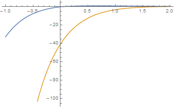
Not too simple, but at least we got it. Let's take a look to see how it did:
enter image description here

Hm, it seems as if our smoothing kernel has had an additional side effect of muliplying our function by a factor of around 100. When we convolve a gaussian with an exponential:

FullSimplify[
 Convolve[Exp[λ x], Exp[-(x/σ)^2/2]/Sqrt[2 Pi]/σ, x, y],
 σ > 0]

the result is the exponential shifted by λ σ^2/2:

E^(y λ + (λ^2 σ^2)/2)

Unfortunately I don't know of a smoothing filter that can avoid this.

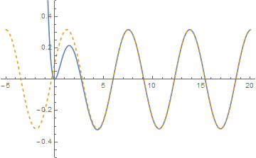
And there is another problem: the fourth term actually cannot be Reduced because its roots are non-analytic. Look what I mean:
enter image description here

The purely sinusoidal part of the term has roots at 2 ArcTan[3 + Sqrt[10]] + Pi C[1], but the exponential part perturbs each root by a small amount. Each of the new roots has no closed-form solution, and each one is shifted by a different amount! Plus, smoothing the sinusoidal part changes the magnitude by a factor of 1/Sqrt[E], probably not what you want. (Again, most smoothing filters will have this type of effect.)

If smoothing the discontinuities is all that you want to achieve, I suggest a different method: modify the term[{a, b}, expr] function to remove the discontinuity at the source!

smoothTerm[{a_, b_}, expr_, scale_: 1] :=
    (a + b (Erf[expr/scale] + 1)/2) expr

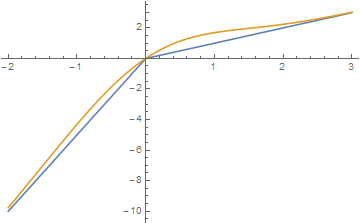
You can replace (Erf[#] + 1)/2 & with whatever smoothing function you want. Here is a comparison of term[{5, -4}, x] and smoothTerm[{5, -4}, x, 3/2]:
enter image description here

I hope you find this useful!

$\endgroup$
0
$\begingroup$

I had to do something similar here: Unable to fit function convolved with NIntegrate with FindFit even with NumericQ (See my answer).

Basically, you need to tell Mathematica to not try to find a symbolic solution and just wait until it can be evaluated numerically using ?NumericQ (there's lots of questions addressing this). Also, I found that it's actually easier to write it in terms of an NIntegrate rather than a Convolve since you you can use AccuracyGoal to make it run way, way faster.

Edit:

f[x_] := Piecewise[{{1, -E^(-2 (x)) + E^-x >= 0}, {0, -E^(-2 (x)) + E^-x <= 0}}]
g[x_] := Piecewise[{{1, -E^(-2 (x)) + 2 E^-x >= 0}, {0, -E^(-2 (x)) + 2 E^-x <= 0}}]
h[x_] := Piecewise[{{1, E^(-2 x)/4 - 2 E^-x + 1/4 (7 - 6 x + 2 x^2) >= 0}, {0, E^(-2 x)/4 - 2 E^-x + 1/4 (7 - 6 x + 2 x^2) <= 0}}]
j[x_] := Piecewise[{{1, (2 E^(-2 x))/5 - E^-x/2 + 1/100 (10 Cos[x] + 30 Sin[x]) >=    0}, {0, (2 E^(-2 x))/5 - E^-x/2 +  1/100 (10 Cos[x] + 30 Sin[x]) <= 0}}]
l[x_] := (-E^(-2 x) + E^-x) (7 - 3 f[x]) + (-E^(-2 x) + 2 E^-x) (2 - 2 g[x]) + (E^(-2 x)/4 - 2 E^-x + 1/4 (7 - 6 x + 2 x^2)) (3 -2 h[x]) + (150 - 100 j[x]) ((2 E^(-2 x))/5 - E^-x/2 +  1/100 (10 Cos[x] + 30 Sin[x]))
Plot[l[x], {x, 0, 25}]

Then define the convolution with a unit gaussian with

Result[x_?NumericQ] :=  NIntegrate[l[x - xp]/Sqrt[2 Pi]*E^(-xp^2/2), {xp, -3, 3},  AccuracyGoal -> 3]

You can get numbers out of this

Result[1.5]

You could plot it using plot, but it takes forever to evaluate each point. However, you can compute the value at say 25 points, and plot those.

Data = Table[{x, Result[x]}, {x, 0, 25, 1}]
ListPlot[Data]

That takes about 4 min to run on my machine. The problem is that your function varies a lot over a gaussian of width 1, and calculating the convolution of a single point even to three digits takes ~ 10 sec.

$\endgroup$
5
  • $\begingroup$ I need the symbolic solution. Because I need to plot the result. $\endgroup$
    – bluehills
    Commented Feb 18, 2015 at 20:49
  • $\begingroup$ You do not need a symbolic solution to plot the result -- I plot the result of mine. $\endgroup$ Commented Feb 18, 2015 at 20:53
  • $\begingroup$ I checked the link you gave. But since I am very fresh in Mathematica, I dont see how I to use NIntegrate in my code. $\endgroup$
    – bluehills
    Commented Feb 18, 2015 at 21:03
  • $\begingroup$ Thanks for your help. I see my function varies that is why I cant get the result of the convolution as a continuous function. Actually what I want is to mollify the function. And for the mollification I need to convolute it with a mollifier. $\endgroup$
    – bluehills
    Commented Feb 18, 2015 at 22:40
  • 1
    $\begingroup$ I think "mollify" is not the word you are looking for? $\endgroup$ Commented Feb 19, 2015 at 16:42

Your Answer

By clicking “Post Your Answer”, you agree to our terms of service and acknowledge you have read our privacy policy.

Not the answer you're looking for? Browse other questions tagged or ask your own question.