Here is an adjacency graph with at least one unconnected node:
am = RandomVariate[BernoulliDistribution[0.1], {9, 9}]

{{0, 0, 0, 0, 0, 0, 0, 0, 0}, {0, 1, 0, 0, 0, 0, 0, 0, 0}, {0, 0, 0,
  0, 0, 0, 0, 1, 0}, {0, 0, 0, 0, 0, 0, 0, 0, 0}, {0, 0, 0, 0, 0, 0,
  0, 0, 0}, {0, 0, 0, 1, 0, 0, 0, 0, 0}, {0, 0, 0, 0, 0, 0, 0, 0,
  1}, {0, 1, 0, 0, 0, 0, 0, 0, 0}, {0, 0, 0, 0, 0, 0, 1, 0, 0}}
Here are the coordinates if you want to lay those nodes out on a grid.
vc = Flatten[Table[{i, j}, {i, 3}, {j, 3}], 1]

{{1, 1}, {1, 2}, {1, 3}, {2, 1}, {2, 2},
{2, 3}, {3, 1}, {3, 2}, {3, 3}}
If you use GraphPlot rather than Graph, the coordinates need to be expressed like this.
vcr = Thread[Range[9] -> vc]

{1 -> {1, 1}, 2 -> {1, 2}, 3 -> {1, 3}, 4 -> {2, 1}, 5 -> {2, 2},
 6 -> {2, 3}, 7 -> {3, 1}, 8 -> {3, 2}, 9 -> {3, 3}}
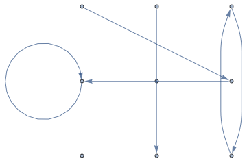
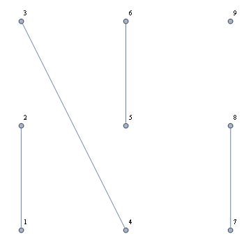
Here is the case using a Graph construct.
AdjacencyGraph[am, VertexCoordinates -> vc]
And here is the case using GraphPlot.
GraphPlot[am, VertexCoordinateRules -> vcr, SelfLoopStyle -> All]
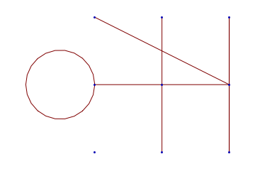
As you can see, if you specify an adjacency matrix, Mathematica will display the unconnected nodes. You can make the nodes easier to see by using options such as VertexSize in Graph, and PlotStyle or VertexRenderingFunction in GraphPlot. Here is an example with GraphPlot where I have also turned off the self-loop:
GraphPlot[am, VertexCoordinateRules -> vcr,
 PlotStyle -> AbsolutePointSize[8]]
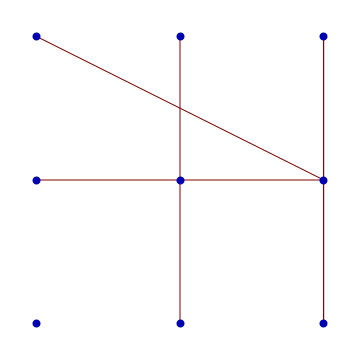
The main difference between Graph and GraphPlot is that the former shows nice curved edges to avoid confusion about whether {1,3} is connected to {3,3} or {2,3}. The option names are all different, too. Which you choose is up to you.

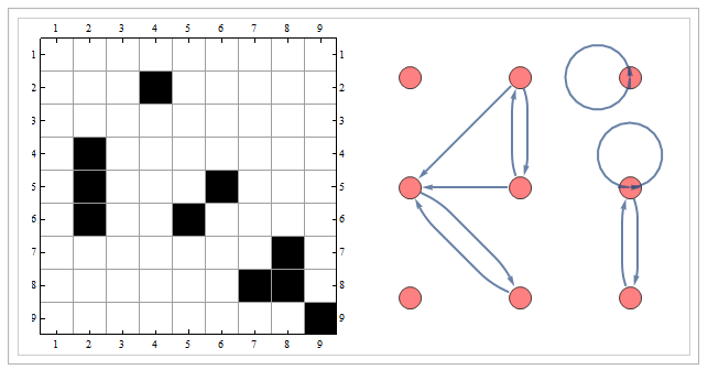


VertexCoordinateswill do what you want. $\endgroup$