50
$\begingroup$

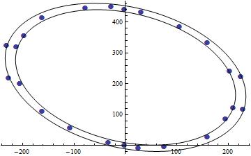
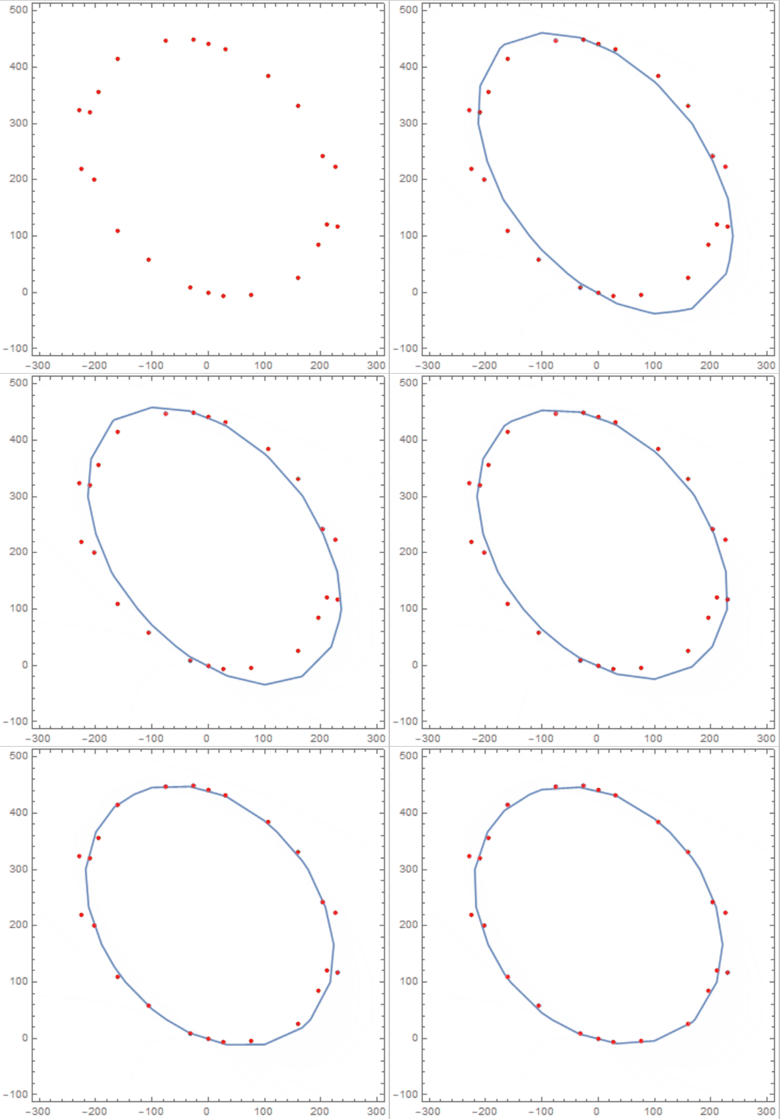
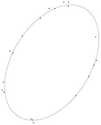
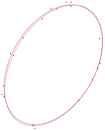
I have 24 x-y points that are supposed to form an ellipse.

points={{31.4799,432.849},{-195.826,356.419},{210.029,121.779},{76.1586,-4.47992},{26.6061,-6.97711},{160.236,27.0398},{203.248,241.865},{-225.351,218.912},{-159.899,109.93},{-106.465,58.164},{-1.98952*10^-11,442.},{-229.146,324.489},{-31.4799,9.15114},{195.826,85.5807},{-210.029,320.221},{-76.1586,446.48},{-26.6061,448.977},{-160.236,414.96},{-203.248,200.135},{225.351,223.088},{159.899,332.07},{106.465,383.836},{-1.98952*10^-11,1.83076*10^-11},{229.146,117.511}};
points//ListPlot
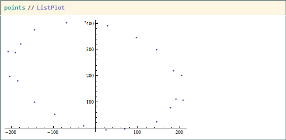
points

I want to numerically fit an ellipse around those points. I tried to use the NMinimize method with least-square shown in this Q&A but the issue in this problem is that x and y are related parametrically (through t), and not directly like that other problem was. Worse, the ellipse will be off-center and tilted, so I can't use the nice $$\left(\frac{x}{a}\right)^2+\left(\frac{y}{b}\right)^2=1$$ but had to use this equation I found on Wikipedia (surprisingly without citation!):

ellipsewiki

My strategy was to generate 24 X(t) equations and 24 Y(t) equations, or more specifically, X(t1), Y(t1), ..., X(t24), X(t24) with xc, yc, a, b in them. Then, I would use NMinimize to optimize all of the square differences between my points and the ellipse. I would eventually get back xc, yc, a, b, CurlyPhi, and every single t values from t1 to t24. I tried to find a more elegant way of using NMinimized for parametric equations, and I believe the multivariate examples of NMinimized in the documentation are not exactly parametric equations. See also the linked Q&A above for an example.

Here's my code to find xc, yc, a, b, t1, ... , t24:

tList = ToExpression["t" <> ToString[#]] & /@ Range[1, 24];
equations = Join[
   MapThread[#1 - xc - a Cos[#2] Cos[φ] + 
      b Sin[#2] Sin[φ] &, {points[[All, 1]], tList}],
   MapThread[#1 - yc - a Cos[#2] Sin[φ] - 
      b Sin[#2] Cos[φ] &, {points[[All, 2]], tList}]];
solution = NMinimize[
  #.# &[equations],
  Join[tList, {xc, yc, a, b, φ}]]
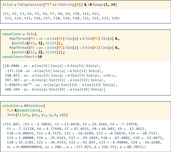
equations

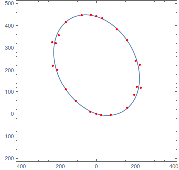
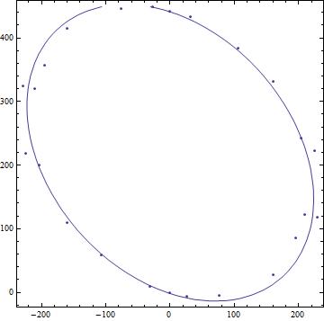
And this is what the ellipse looks like:

Show[

 (* Tilted ellipse/disk drawn using Disk and Rotate *)
 Graphics[
  {Yellow, 
   Rotate[Disk[{xc, yc}, {Abs@a, b}], φ] /. 
    solution[[2, 25 ;; 29]]}],

 (* Starting points *)
 points // ListPlot,

 (* Ellipse outline plotted by the 2 parametric equations *)
 ParametricPlot[{xc + a Cos[t] Cos[φ] - 
     b Sin[t] Sin[φ], 
    yc + a Cos[t] Sin[φ] + b Sin[t] Cos[φ]} /. 
   solution[[2, 25 ;; 29]], {t, 0, 2 π}, PlotStyle -> Red],

 (* Point on ellipse corresponding to t1 to t24 *)
 ListPlot[{xc + a Cos[#] Cos[φ] - b Sin[#] Sin[φ],
       yc + a Cos[#] Sin[φ] + b Sin[#] Cos[φ]} /. 
     solution[[2, 25 ;; 29]] & /@ solution[[2, 1 ;; 24, 2]], 
  PlotStyle -> Red],

 Axes -> True]
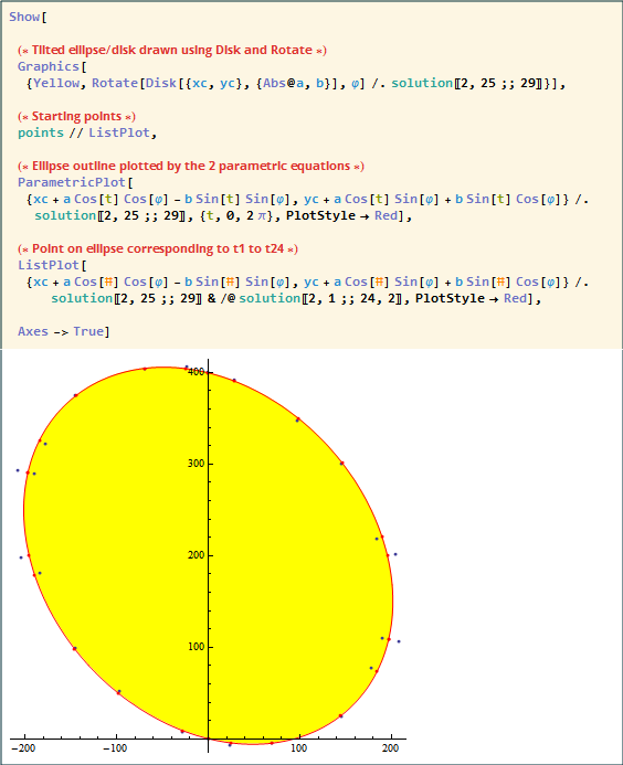
ellipse

Even though I got what I want, I just feel that this is clunky way to solve the problem, not least because I don't need to solve for t1 to t24--I just needed xc, yc, a, and b. Another issue is that for some reason the value of my a (supposed to be the long axis) is negative and smaller in magnitude than the other axis*, and the rotate angle of the ellipse is crazy high (88.7 radian). I tried to apply some constrains to NMinimize (a>0 or 90 ° < φ < 150 °) but kept getting errors.
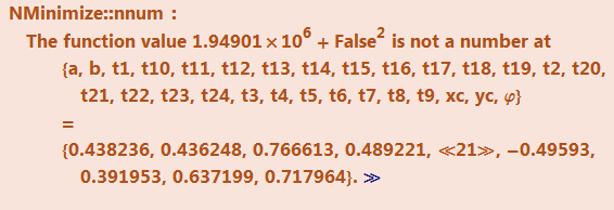
NMinimized error

*

ellipse wiki reference

Lastly, I'd really appreciate any general comment to make my code better as I'm still a beginner in MMA (you probably could tell by my zeal of pure functions in this example; I've just been reading a chapter about them).

$\endgroup$
6
  • 4
    $\begingroup$ This might be interesting for you: link $\endgroup$
    – eldo
    Commented Jun 25, 2014 at 11:28
  • 1
    $\begingroup$ i did this some years ago as a two level fit algorithm. Estimate xc,yc. Transform data to polar coordinates and use NonlinerarModelFit to fit the three parameters a,b,phi to the polar ellipse equation. Wrap that in a fit to optimize the center position. (my experience this worked far better than a direct 5 parameter fit) $\endgroup$
    – george2079
    Commented Jun 25, 2014 at 12:44
  • 2
    $\begingroup$ (1) There are a number of approaches posted that seem good. About the only thing to be on the alert for is a "solution" that actually gives a hyperbola. This can happen in extreme cases of troublesome data. So you may want to enforce an inequality constraint in any optimization. $\endgroup$ Commented Jun 25, 2014 at 18:41
  • 4
    $\begingroup$ (2) Also maybe have a look at "Direct and specific least-square fitting of hyperbolae and ellipses" by P. O'Leary and P. Zsomber-Murray, Journal of Electronic Imaging 13:492-503, 2004. $\endgroup$ Commented Jun 25, 2014 at 18:42
  • 1
    $\begingroup$ See also the well-written description of ellipse parameters at mathworld.wolfram.com/Ellipse.html $\endgroup$
    – John McGee
    Commented Jul 2, 2014 at 10:47

8 Answers 8

46
$\begingroup$

Here is another approach. It could be improved (I am sure) to properly determined the principle axes and translation (if I get time I will aim to update):

lin = {#1^2, #1, #2, 2 #1 #2, #2^2} & @@@ points;
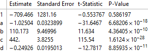
lm = LinearModelFit[lin, {1, a, b, c, d}, {a, b, c, d}]

Exploring model:

lm["ParameterTable"]

enter image description here

Determining quadric formula:

pa = lm["BestFitParameters"];
w[x_, y_] := pa.{1, x^2, x, y, 2 x y} - y^2;
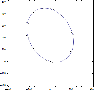
ContourPlot[w[x, y] == 0, {x, -400, 400}, {y, -200, 500}, 
 Epilog -> Point[points]]

enter image description here

Formula:

TraditionalForm[-w[x, y] == 0]

enter image description here

UPDATE

I post this update to determine the translation from origin, the principle axes and the $a$ and $b$ of the desired form $\frac{x^2}{a^2}+\frac{y^2}{b^2}=1$ and hence assessment of area of ellipse: viz $\pi a b$ etc. The axes can be swapped as desired.

The translation can be derived as follows:

{dx, dy} = 
 0.5 Inverse[{{-pa[[2]], -pa[[5]]}, {-pa[[5]], 1}}].{pa[[3]], pa[[4]]}

yielding:

{0.0000180983, 221.}

The axes can be derived from the matrix of quadric form:

mat = {{-pa[[2]], -pa[[5]]}, {-pa[[5]], 1}};
const = (-pa[[2]] dx^2 + dy^2 - 2 pa[[5]] dx dy) - pa[[1]]
trf[x_, y_] := -pa[[2]] (x - dx)^2 - 
  2 pa[[5]] (x - dx) (y - dy) + (y - dy)^2 - const

Then translating ellipse back to origin:

tran = Simplify@trf[x + dx, y + dy]

yields:

-49550.5 + 1.02504 x^2 + 0.498521 x y + y^2=0

Then looking at the eigensystem of matrix will allow visualization of principal axes:

fun[poly_, a_] := Module[{mat, val, vc, vcn, gr},
   mat = {{#1, #2/2}, {#2/2, #3}} & @@ (Coefficient[
       poly, {x^2, x y, y^2}]);
   {val, vc} = Eigensystem[mat];
   vcn = Normalize /@ vc;
   gr = Graphics[{Line[{{0, 0}, Sqrt[a] vcn[[1]]/Sqrt[Abs@val[[1]]]}],
       Line[{{0, 0}, Sqrt[a] vcn[[2]]/Sqrt[Abs@val[[2]]]}]}];
   Show[ContourPlot[poly == a, {x, -500, 500}, {y, -500, 500}], gr]
   ];

The values of $a$ and $b$ can e derived:

{ev, vec} = Eigensystem[mat];
st = {x^2, y^2}.ev;
{a, b} = Sqrt[1/Coefficient[Expand[st/const], {x^2, y^2}]]

yields:

{198.143, 254.846}

Putting visualizations all together:

cntr = ContourPlot[trf[x, y] == 0, {x, -500, 500}, {y, -200, 500}, 
  Epilog -> {Point[points], {Red, PointSize[0.03], Point[{dx, dy}]}}];
axes = fun[1.0250354570455185` x^2 + 0.49852055996040495` x y + y^2, 
  49550.46446156194`];
norm = ContourPlot[st == const, {x, -500, 500}, {y, -500, 500}];

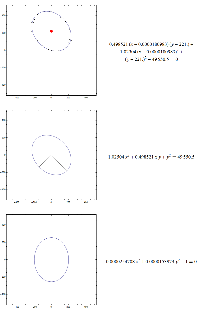
These graphics and corresponding equations were threaded then exported as an animated gif:

grap = Show[#, PlotRange -> {{-500, 500}, {-500, 500}}] & /@ {cntr, 
   axes, norm}
eqns = Style[#, 20] & /@ {TraditionalForm[trf[x, y] == 0], 
   TraditionalForm[
    1.0250354570455185` x^2 + 0.49852055996040495` x y + y^2 == 
     49550.46446156194`], TraditionalForm[ell[x, y] == 0]}

enter image description here

The gif cycles through (i) data with fit and red point is {dx,dy} (ii) the second is the ellipse translated to the origin (iii) the ellipse axes are 'aligned' to cartesian axes.

$\endgroup$
7
  • 1
    $\begingroup$ Beautifully terse. You could make it more so with {#^2, ##, 2 ##, #2^2} & @@@ points. :-) $\endgroup$
    – Mr.Wizard
    Commented Jun 25, 2014 at 16:09
  • $\begingroup$ @Mr.Wizard thank you for kind comment, edit and education $\endgroup$
    – ubpdqn
    Commented Jun 26, 2014 at 9:30
  • $\begingroup$ Could you provide a reference for {dx, dy} = 0.5 Inverse[{{-pa[2], -pa[[5]]}, {-pa[[5]], 1}}].{pa[3], pa[4]}? I'm struggling to find a way to convert between general formula of an ellipse (x^2,y^2,xy,...) to the form that shows a and b. $\endgroup$ Commented Jun 26, 2014 at 19:26
  • $\begingroup$ @seismatica {dx,dy} is just equating coefficients: $ax^2+bx+2cxy++dy+y^2= a(x-dx)^2+2c(x-dx)(y-dy)+(y-dy)^2-a dx^2-dy^2-2dx dy$ just solving using linear algebra. Daniel Lichtblau;s answer is a professional general way cf my hamfisted approach. $\endgroup$
    – ubpdqn
    Commented Jun 26, 2014 at 22:50
  • $\begingroup$ This worked well for the points in the example, but not for these: {{354.7, 167.5}, {349.7, 190.}, {347.6, 198.2}, {321.2, 233.3}, {279., 254.}, {246.8, 255.}, {232.4, 247.7}, {214., 234.5}, {189.7, 182.1}, {186.1, 174.}, {183.2, 166.1}, {187.6, 128.1}, {229.2, 94.}, {232.4, 91.7}, {281.8, 84.9}, {302.3, 87.9}, {322.1, 95.7}, {344.8, 124.6}, {352.2, 146.}} It seemed to work with the following changes: mat = {{Abs[pa[[2]]], Abs[pa[[5]]]}, {Abs[pa[[5]]], 1}} and const = (-pa[[2]] dx^2 + dy^2 - 2 pa[[5]] dx dy) + pa[[1]] but I don't really understand why... can anyone confirm? $\endgroup$
    – MelaGo
    Commented Mar 12, 2019 at 22:33
32
$\begingroup$

Here is a standard direct way to get the principal exes and other transformation data. Find the mean of the points, subtract it to center them, and take the singular value decomposition. The third and second components thereof give the rotation and scaling data necessary to form a circle on which the first component, viewed as a point set, roughly lies. The average distance from origin of this new point set gives a radius. Now invert all that to get the ellipse equation.

While I'm sure that made no sense (least of all to me), the coding is straightforward.

mean = Mean[points];
newpts = Map[# - mean &, points];
{uu, ww, vv} = SingularValueDecomposition[newpts, 2]

(* Out[195]= {{{0.154787303139, 
   0.24681671674}, {0.264618646868, -0.0802782275335}, \
{-0.244940409458, 
   0.132178292936}, {-0.2488804106, -0.141810231081}, \
{-0.21297321559, -0.198934383898}, {-0.286761033433, \
-0.0175688333828}, {-0.138307266939, 
   0.244940128897}, {0.171124630754, -0.250504589808}, \
{0.0288583749054, -0.287472943299}, {-0.0558601605337, \
-0.280401389223}, {0.186667941, 
   0.221277578296}, {0.263211882778, -0.148978381541}, \
{-0.154787157436, -0.246816544024}, {-0.264618872812, 
   0.0802779596975}, {0.244940436909, -0.132178260395}, \
{0.248880505624, 0.141810343723}, {0.21297315013, 
   0.1989343063}, {0.286760891953, 
   0.0175686656724}, {0.13830729439, -0.244940096356}, \
{-0.171124603303, 0.250504622349}, {-0.0288583474542, 
   0.28747297584}, {0.0558601879848, 
   0.280401421764}, {-0.186667913548, -0.221277545756}, \
{-0.263211855327, 0.148978414082}}, {{876.375887309, 0.}, {0., 
   671.508170856}}, {{-0.672351542658, 
   0.740231992746}, {0.740231992746, 0.672351542658}}} *)

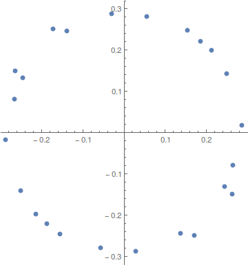
Here is the circle, centered at the origin, that the new points (from the left factor, uu), occupy.

ListPlot[uu, AspectRatio -> Automatic]

enter image description here

Now get the radius squared of this new circle.

rsqr = Mean[Map[#.# &, uu]]

(* Out[191]= 0.0833333333333 *)

To get to this origin-centered circle we run the transformations on our variables, {x,y}, to get new coordinates in terms thereof.

{nx, ny} = Inverse[vv.ww].({x, y} - mean);

So here is the ellipse equation.

expr = Expand[nx^2 + ny^2] == rsqr

(* Out[201]= 
0.0838086622042 - 0.000201425757605 x + 1.80374774713*10^-6 x^2 - 
  0.00075844948748 y + 9.11428834461*10^-7 x y + 
  1.71594919287*10^-6 y^2 == 0.0833333333333 *)

We'll check this pictorially.

ContourPlot[Evaluate@expr, {x, -400, 400}, {y, -200, 500}, 
 Epilog -> {Red, PointSize[Medium], Point[points]}]

enter image description here

$\endgroup$
4
  • $\begingroup$ I certainly enjoyed reading your code. Elegant and understandable. $\endgroup$
    – eldo
    Commented Jun 25, 2014 at 20:26
  • $\begingroup$ @DanielLichtblau thank you for such a clear exposition of the linear algebra...closer and general cf contortions (which really use linear algebra in a tortured way) $\endgroup$
    – ubpdqn
    Commented Jun 26, 2014 at 21:49
  • $\begingroup$ But what if the points are not uniformly distributed around the ellipse, but skewed to one side? For example, what if they all lie on a partial elliptic arc? $\endgroup$
    – Szabolcs
    Commented Oct 16, 2018 at 14:29
  • $\begingroup$ @Szabolcs I have not done experiments. My guess is it would not work well for that case. I'd have to think through the math to be sure though. Linear least-squares would still work fine though. $\endgroup$ Commented Oct 16, 2018 at 20:59
22
$\begingroup$

The approach mentioned in my comment using a polar representation:

 r[a_, b_, theta_, t_] := 
      a Sqrt[2]/Sqrt[ (1 + (a/b)^2) + (1-(a/b)^2) Cos[2 (t - theta)] ];

some random sample data:

 data = With[ {a = 1, b = 1/2, theta = Pi/3 , x0 = 1, y0 = 1} ,
     Table[{x0, y0} + {Cos[t], Sin[t] } r[a, b, theta, t] +
     RandomVariate[NormalDistribution[0, .05], 2] ,
       {t, RandomVariate[UniformDistribution[{0, 2 Pi}], 100]} ]];

polar coordinate fit about a given center:

bestpfit[{xc_?NumericQ, yc_?NumericQ}, data_] := Module[{polardata,fit},
  polardata = { ArcTan @@ # , Norm[#] } & /@ ( # - {xc, yc} & /@ data);
  fit = NonlinearModelFit[ polardata, 
        r[ a, b, theta, t] , {a, b, theta } , { t} ];
  param = fit["BestFitParameters"];
  Norm@fit["FitResiduals"] ]

it helps to make a good guess at the center..then find xo,y0 to minimize the residual of the polar fit:

 guess = Mean[data];
 min = FindMinimum[ 
   bestpfit[{x0, y0}, data] , {{x0, guess[[1]]}, {y0, guess[[2]]}}] ;
 result = param~Join~min[[2]]

( note param is a global set by the last call to bestpfit .. probably there is a better way to do that )

{a -> 0.988222, b -> 0.475728, theta -> 0.990139, x0 -> 1.01157, y0 -> 1.00329}

(recall input was {1,1/2,1.0472,1,1})

 Show[{ListPlot[data, PlotStyle -> Red], 
      ParametricPlot[ {x0, y0} + {Cos[t], Sin[t] } r[a, b, theta, t] /. 
        result , {t, 0, 2 Pi}]}, PlotRange -> All]

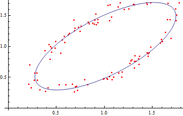
enter image description here

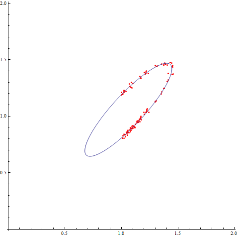
This works well even with data not fully populating the ellipese:

 data = Select[ With[ {a = 1, b = 1/10, theta = Pi/6 , x0 = 1, y0 = 1} ,
      Table[{x0, y0} + {Cos[t], Sin[t] } r[a, b, theta, t] +
         RandomVariate[NormalDistribution[0, .01], 2] ,
           {t, RandomVariate[UniformDistribution[{0, 2 Pi}], 
                200]} ]] , #[[1]] > 1 && #[[2]] > 1/2 & ];

enter image description here

$\endgroup$
8
  • $\begingroup$ You've got my vote. I'm not sure why nobody else seems to have noticed this answer. $\endgroup$
    – Mr.Wizard
    Commented Jun 25, 2014 at 17:57
  • $\begingroup$ You said in your comment that "this worked far better than a direct 5 parameter fit" in your experience. Can you elaborate a little on why that might be, or in what cases would this approach work better than the simpler direct fit? $\endgroup$
    – user484
    Commented Jun 25, 2014 at 18:45
  • $\begingroup$ It may well be that my 5 parameter algorithm wasn't very good (!). That was long ago and w/o mathematica. I'm sure the issue was fit success, not performance though. If I had time I'd try the other answers here on my last poor-data example.. $\endgroup$
    – george2079
    Commented Jun 25, 2014 at 19:10
  • $\begingroup$ George2079 could you ellaborate on how you got the polar ellipse equation with tilt in the first place? It looks a good method though! $\endgroup$
    – user34792
    Commented Oct 13, 2015 at 15:28
  • $\begingroup$ @Elliet I don't know where I got that but it wasn't even right. (corrected). You can find that basic formula on the wikipedia ellipse page. $\endgroup$
    – george2079
    Commented Oct 13, 2015 at 17:59
21
$\begingroup$

In analytic geometry, the ellipse is defined as the set of points (X,Y) of the Cartesian plane that, in non-degenerate cases, satisfy the implicit equation enter image description here

with enter image description here and enter image description here where

enter image description here

enter image description here

enter image description here

Lets fit points with second-order curve (which include ellipse).

elipse = a11*x^2 + a22*y^2 + 2*a12*x*y + 2*a13*x + 2*a23*y + a33;
coeff = {a11, a22, a12, a13, a23, a33};
fitResult=FindFit[points/.{x_,y_}:>{x,y,0},{elipse,{#>0||#<0}&/@coeff},coeff,{x,y}];
elipse=elipse/.fitResult
(*{a11->0.002852802341,a22->0.002611181564,a12->0.0008537122851,a13->-0.188169993,a23->-0.5733778586,a33->-2.326357837}*)

Then check result

Show[{ContourPlot[res==0,{x,Min[points],Max[points]},{y,Min[points],Max[points]}],ListPlot[points]},PlotRange->All]

enter image description here

$\endgroup$
1
  • 3
    $\begingroup$ It becomes easier, and stabler, if you get rid of a23 and instead force the constant to be 1. $\endgroup$ Commented Jun 26, 2014 at 0:06
20
$\begingroup$
Needs["MultivariateStatistics`"]

points = {{31.4799, 432.849}, {-195.826, 356.419}, {210.029, 
    121.779}, {76.1586, -4.47992}, {26.6061, -6.97711}, {160.236, 
    27.0398}, {203.248, 241.865}, {-225.351, 218.912}, {-159.899, 
    109.93}, {-106.465, 58.164}, {-1.98952*10^-11, 442.}, {-229.146, 
    324.489}, {-31.4799, 9.15114}, {195.826, 85.5807}, {-210.029, 
    320.221}, {-76.1586, 446.48}, {-26.6061, 448.977}, {-160.236, 
    414.96}, {-203.248, 200.135}, {225.351, 223.088}, {159.899, 
    332.07}, {106.465, 383.836}, {-1.98952*10^-11, 
    1.83076*10^-11}, {229.146, 117.511}};

Show[ListPlot[points, PlotMarkers -> {Automatic, Medium}], 
 Graphics[EllipsoidQuantile[points, {0.1, 1.}]], PlotRange -> All]

enter image description here

$\endgroup$
1
  • $\begingroup$ Very underrated (under-voted) answer! $\endgroup$ Commented Nov 22, 2020 at 14:16
15
$\begingroup$

Here is a Neural Networks' way to solve this question.

Wiki says the equation of Eclipse is:

$A x^2+B x y+C y^2+D x+E y+F=0$

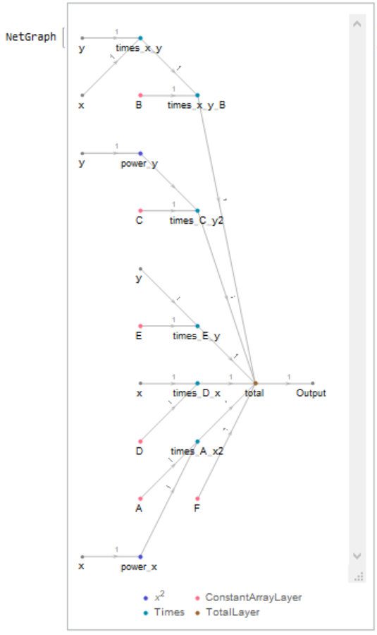
Firstly,defining the net that equal this equation

net = NetGraph[<|"power_x" -> ElementwiseLayer[#^2 &], 
                 "power_y" -> ElementwiseLayer[#^2 &], 
                 "times_x_y" -> ThreadingLayer[Times], 
                 "times_x_y_B" -> ThreadingLayer[Times], 
                 "times_A_x2" -> ThreadingLayer[Times], 
                 "times_C_y2" -> ThreadingLayer[Times], 
                 "times_D_x" -> ThreadingLayer[Times], 
                 "times_E_y" -> ThreadingLayer[Times], 
                 "A" -> ConstantArrayLayer["Array" -> {1}], 
                 "B" -> ConstantArrayLayer["Array" -> {1}], 
                 "C" -> ConstantArrayLayer["Array" -> {1}], 
                 "D" -> ConstantArrayLayer["Array" -> {1}], 
                 "E" -> ConstantArrayLayer["Array" -> {1}], 
                 "F" -> ConstantArrayLayer["Array" -> {1}], 
                 "total" -> TotalLayer[]|>, 
                 {NetPort["x"] -> "power_x", {"power_x", "A"} -> "times_A_x2" -> "total", 
                  NetPort["y"] -> "power_y", {"power_y", "C"} -> "times_C_y2" -> "total", 
                  {NetPort["x"], NetPort["y"]} -> "times_x_y", {"times_x_y", "B"} -> "times_x_y_B" -> "total", 
                 {"D", NetPort["x"]} -> "times_D_x" -> "total", 
                 {"E", NetPort["y"]} -> "times_E_y" -> "total", 
                  "F" -> "total"}]

enter image description here

Transforming the original data to net format.

data = <|"x" -> List /@ #[[All, 1]], "y" -> List /@ #[[All, 2]], 
         "Output" -> List /@ ConstantArray[0, Length@#]|> &@points

Training the net.

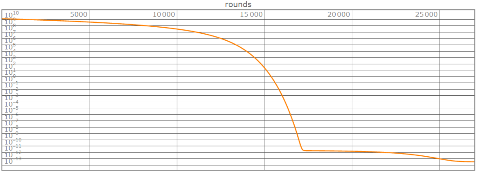
{net, img} = NetTrain[net, data, MeanSquaredLossLayer[], 
                     {"TrainedNet", "LossEvolutionPlot"}, 
                      Method -> {"ADAM", "InitialLearningRate" -> 0.0001}, 
                      MaxTrainingRounds -> 27000];

enter image description here

Got the coefficient of Eclipse:

{a, b, c, d, e, f} = Flatten[NetExtract[net, {#, "Array"}] & /@ {"A", "B", "C", "D", "E", "F"}]

{-1.83805*10^-10, -8.56689*10^-11, -1.66141*10^-10, 1.86014*10^-8, 7.17712*10^-8, 7.61086*10^-7}

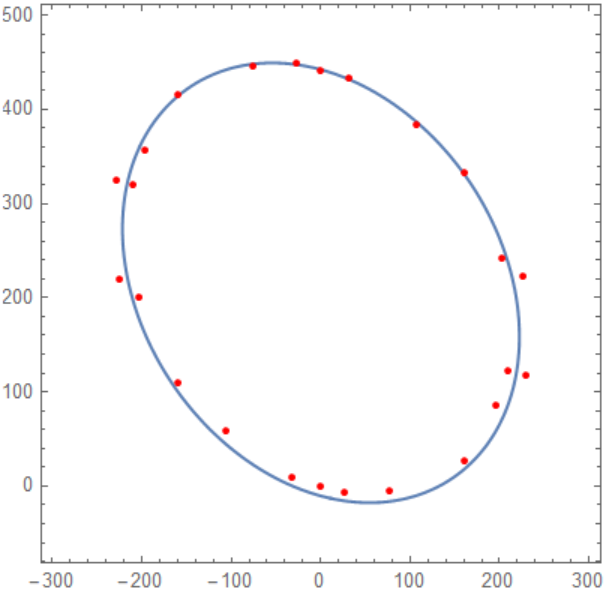
The curve of eclipse and data points coincide.

Show[ContourPlot[{a*x^2 + b*x*y + c*y^2 + d*x + e*y + f == 0}, {x, -300, 300}, {y, -100, 500}, PlotPoints -> 50], 
     ListPlot[points,PlotStyle -> Red]]

enter image description here

Update:Using this code can get a gif about how the net fitting the data

plotSolution[weightsAss_] := Module[{temp =Flatten@Values@KeySort[weightsAss]}, 
   Show[ContourPlot[{temp[[1]]*x^2 + temp[[2]]*x*y + temp[[3]]*y^2 + 
   temp[[4]]*x + temp[[5]]*y + temp[[6]] == 0}, {x, -300, 300}, {y, -100, 500}], 
   ListPlot[points, PlotStyle -> Red]]]

net = NetTrain[net, data, 
      Method -> {"ADAM", "InitialLearningRate" -> 0.0001}, 
      MaxTrainingRounds -> 27000, 
      TrainingProgressReporting -> {plotSolution[#Weights] &, "Interval" -> 0.1}];

After a while you can see the animation~ have fun~~~

enter image description here

$\endgroup$
2
  • $\begingroup$ First thing I've ever seen that made me want to learn something about Neural Nets. $\endgroup$
    – Reb.Cabin
    Commented May 6, 2019 at 1:54
  • $\begingroup$ @Reb.Cabin :-) It will be an amazing adventure! $\endgroup$
    – partida
    Commented May 6, 2019 at 5:32
6
$\begingroup$

Background

Let us derive a method that generalizes straightforwardly for arbitrary dimensional ellipsoids.

The implicit equation of an ellipse can be written as

$$ (r-r_0)^T A (r-r_0)=1$$

where the $r_0$ vector is the centre of the ellipse and $A$ is a symmetric positive definite matrix. The eigenvalues of $A$ give the inverse squared semi-major and semi-minor axes. The eigenvectors of the matrix are orthogonal to each other (since $A$ is symmetric) and give the directions of the axes of the ellipse.

Inverse[A] is the matrix used in the second argument of Ellipsoid.

Derivation

Expanding the above equation, and keeping in mind that $A^T=A$, we get

$$ r^T A r - 2 r_0^T A r + r_0^T A r_0 = 1 $$

We can get rid of the constant term $r_0^T A r_0$ by making the substitution $A = B / (1 + r_0^T B r_0)$, and finally obtaining

$$ r^T B r - 2 r_0^T B r = 1.$$

Let us write the equation for the two-dimensional case in terms of the explicit coordinates $r = (x,y)$. It will be the linear combination of five terms:

$$a x^2 + b y^2 + c (2xy) + d x + e y = 1.$$

The coefficients $a,b,c,d,e$ can be obtained using linear regression (e.g. LeastSquares). Once we have them, we need to compute $B$ and $r_0 = (x_0, y_0)$.

By matching up the elements of the matrix $B$ with the coefficients, we get

$$B = \left(\begin{array}{cc} a & c \\ c & b \end{array}\right),$$

Then we can compute $r_0$ by solving the linear equation $-2B r_0 = \binom{d}{e}$.

Implementation

The implementation is straightforward.

fitEllipse[pts_] :=
 Module[{lsMat, a, b, c, d, e, A, B, r0},
   lsMat = Function[{x, y}, {x^2, y^2, 2 x y, x, y}] @@@ pts;
   {a, b, c, d, e} = LeastSquares[lsMat, ConstantArray[1, Length[pts]]];
   B = {{a, c}, {c, b}};
   r0 = LinearSolve[-2 B, {d, e}];
   A = B/(1 + r0.B.r0);
   Ellipsoid[r0, Inverse[A]]
 ]

Demonstration:

ellipse = Ellipsoid[{1, 2}, {{2, 1}, {1, 3}}];

n = 20;
pts = RandomPoint[RegionBoundary[ellipse], n] + RandomVariate[NormalDistribution[0, 0.05], {n, 2}];

Sadly, displaying Ellipsoid in Graphics is buggy in M11.3, so we need to use BoundaryDiscretizeRegion to display it correctly.

Show[
 BoundaryDiscretizeRegion[ellipse, MeshCellStyle -> {2 -> None}], 
 Graphics[{Point[pts]}]
]

enter image description here

fittedEllipse = fitEllipse[pts]
(* Ellipsoid[{0.981358, 2.02406}, {{2.00737, 0.921653}, {0.921653, 2.94451}}] *)

Show[
 BoundaryDiscretizeRegion[ellipse, MeshCellStyle -> {2 -> None}],
 BoundaryDiscretizeRegion[fittedEllipse, MeshCellStyle -> {2 -> None, 1 -> Red}],
 Graphics[{Point[pts]}]
]

enter image description here

We can get the semi-major and semi-minor axes as

Sqrt@Eigenvalues@Last[ellipse]

and the rotation matrix as

Transpose[Normalize /@ Eigenvectors@Last[ellipse]]

Based on this, here's another workaround function for displaying an Ellipsoid correctly.

renderEllipse[Ellipsoid[r0_, A_?MatrixQ]] :=
 Module[{eval, evec},
  {eval, evec} = Eigensystem@N[A]; (* numeric (!!) eigenvalues are already normalized *)  
  GeometricTransformation[
    Circle[{0, 0}, Sqrt[eval]],
    Composition[TranslationTransform[r0], AffineTransform@Transpose[evec]]
  ]
 ]

Then use Graphics[{Point[pts], renderEllipse[fittedEllipse]}].

$\endgroup$
1
$\begingroup$

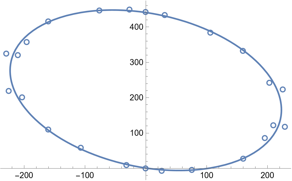
As of 2023.9.15, we can use ResourceFunction["EllipseFit"] for the task:

plot = ListPlot[points, PlotMarkers -> "OpenMarkers"];

eq = ResourceFunction["EllipseFit"][points, {x, y}]
(* -317.095 + 72.414 x - 0.679238 x^2 + 290.267 y - 0.327665 x y - 
  0.656712 y^2 == 0 *)

plot~Show~ContourPlot[eq // Evaluate, {x, #, #2}, {y, #3, #4}] & @@ 
 Flatten@CoordinateBounds@points

enter image description here

$\endgroup$

Not the answer you're looking for? Browse other questions tagged or ask your own question.