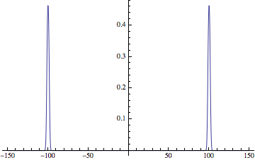
The integrand is nearly zero except for two maxima near -100 and 100. For some reason I do not understand, changing the precision causes the sampling to miss the rather small regions where the integrand is significantly greater than zero. (Changing the precision changes the calculations, and perhaps that is the whole reason.)
A fix would be to control the sampling to include the peaks.
Illustration of the sampling
Here is a look at the function and value away from peaks -- the value is quite small!:
f[x_] := (1/2) PDF[NormalDistribution[-100, 1], x] +
         (1/2) PDF[NormalDistribution[+100, 1], x]

Plot[f[x] Log2[1/f[x]], {x, -150, 150}, PlotRange -> All]
{f[10], f'[10]} // N
(*
   {2.554043924441158*10^-1760, 2.298639531997042*10^-1758}
*)
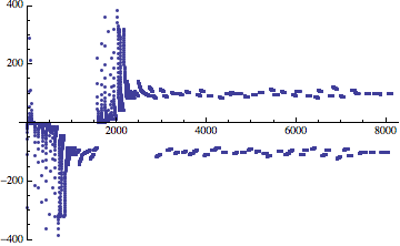
Here is a look at the sampling for two settings of WorkingPrecision, using Sow to stored each value of x at which the integrand is evaluated:
g[n_] := NIntegrate[f[x] Log2[1/f[x]], {x, -Infinity, Infinity},
   MaxRecursion -> 20, WorkingPrecision -> n,
   EvaluationMonitor :> Sow[x]];

{int, samp} = Reap @ g[62];
int
ListPlot[samp, PlotRange -> {-400, 400}]
(*
   3.0470955851806411027016019880549497362225614404580137317711359
*)
{int, samp} = Reap @ g[63];
int
ListPlot[samp, PlotRange -> {-400, 400}]
(*
1.52354779259032055135080099402747486811128072022900686588556600
*)
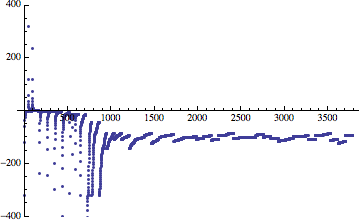
We can see above that the first integral found both maxima and the second found only one. Mathematica estimates the error from the function evaluations (perhaps from its derivatives, too -- I'm ignorant of the actual workings). If it misses a peak and all the values are extremely close to zero, it's likely that the estimate of the error would be nearly zero.
One thing to notice is that the sampling is biased. Initial sampling starts near zero and grows exponentially.
Getting NIntegrate to include the peaks
This has to be done "by hand" in some sense. If you know about where the peaks are, you can use FindMaximum to get closer to them. If it isn't known where they all are, then it may be that not enough is known yet to solve the problem.
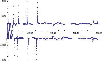
As Stephen Luttrell points out in a comment, you can specify extra points in the domain. These are tested to see if there are singularities, but even if this function passes the test, the side effect is that the peaks are included in the sampling.
g2[n_] :=
 NIntegrate[f[x] Log2[1/f[x]], {x, -Infinity, -100, 100, Infinity},
  PrecisionGoal -> Automatic, WorkingPrecision -> n,
  EvaluationMonitor :> Sow[x]]

{int, samp} = Reap@g2[63];
int
ListPlot[samp, PlotRange -> {-400, 400}]
(*
   3.04709558518064110270160198805494973622256144045801373177111896
*)
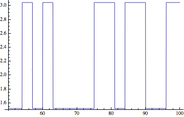


g[n_] := NIntegrate[f[x] Log2[1/f[x]], {x, -Infinity, Infinity}, Method -> "DoubleExponential", MaxRecursion -> 20, WorkingPrecision -> n]seems more reliable. $\endgroup$NIntegrate[ f[x] Log2[1/f[x]], {x, -\[Infinity], -100, 100, \[Infinity]}]andNIntegrate[f[x] Log2[1/f[x]], {x, -\[Infinity], \[Infinity]}]. By using the{x, x1, x2, ..., xn}form for the range of integration (see the documentation "Details"for NIntegrate) to suggest the location of the "singularities",NIntegratecan then compute the correct result. $\endgroup$