Unable to solve the expontial equations [duplicate]

Question

eq1 = 0.013* 
   I0 *(Integrate[Exp[x/Attc], {x, 0, Tc}] + 
      Integrate[Exp[x/Attc], {x, Tge, Tge + 2 Tc}]*Exp[Tc/Attc]*
       Exp[Tge/Attge] )/(0.019 * I0 *
      Integrate [Exp[x/Attge], {x, Tc, Tc + Tge}]*Exp[Tc/Attc]) == 
  0.25/0.38

eq3 = Attge == 2.3

eq4 = Attc ==  2.0

Solve[{eq1,eq3,eq4}, Tc]

I just want to get the relation between Tc and Tge. I dont know why it keeps saying Solve::inex: Solve was unable to solve the system with inexact coefficients or the system obtained by direct rationalization of inexact numbers present in the system. Since many of the methods used by Solve require exact input, providing Solve with an exact version of the system may help. >>

Thanks for any help.

Answer 1

Duplicate or not, but the equation, eq1, is too complex for Mathematica to be solved analytically. Anyway I would first look at the solution. First make the integration in the left-hand part of eq1:

     0.013*I0*(Integrate[Exp[x/Attc], {x, 0, Tc}] + 
         Integrate[Exp[x/Attc], {x, Tge, Tge + 2 Tc}]*Exp[Tc/Attc]*
          Exp[Tge/Attge])/(0.019*I0*
         Integrate[Exp[x/Attge], {x, Tc, Tc + Tge}]*
         Exp[Tc/Attc]) // Simplify

   (* (0.684211 E^(-0.934783 Tc) (-2. + 2. E^(0.5 Tc) + 
       E^(0.5 Tc + 0.934783 Tge) (-2. + 2. E^(1. Tc))))/(-2.3 + 
     2.3 E^(0.434783 Tge))  *)

and then plot it:

    Attge = 2.3;
Attc = 2.0;
Manipulate[
 Plot[(0.68 E^(-0.935 Tc) (-2.` + 2.` E^(0.5` Tc) + 
     E^(0.5` Tc + 0.935 Tge) (-2. + 2.` E^(1. Tc))))/(-2.3 + 
   2.3 E^(0.435 Tge)), {Tc, 0, 10}], {Tge, 1, 50}]

You should be able to see the following: 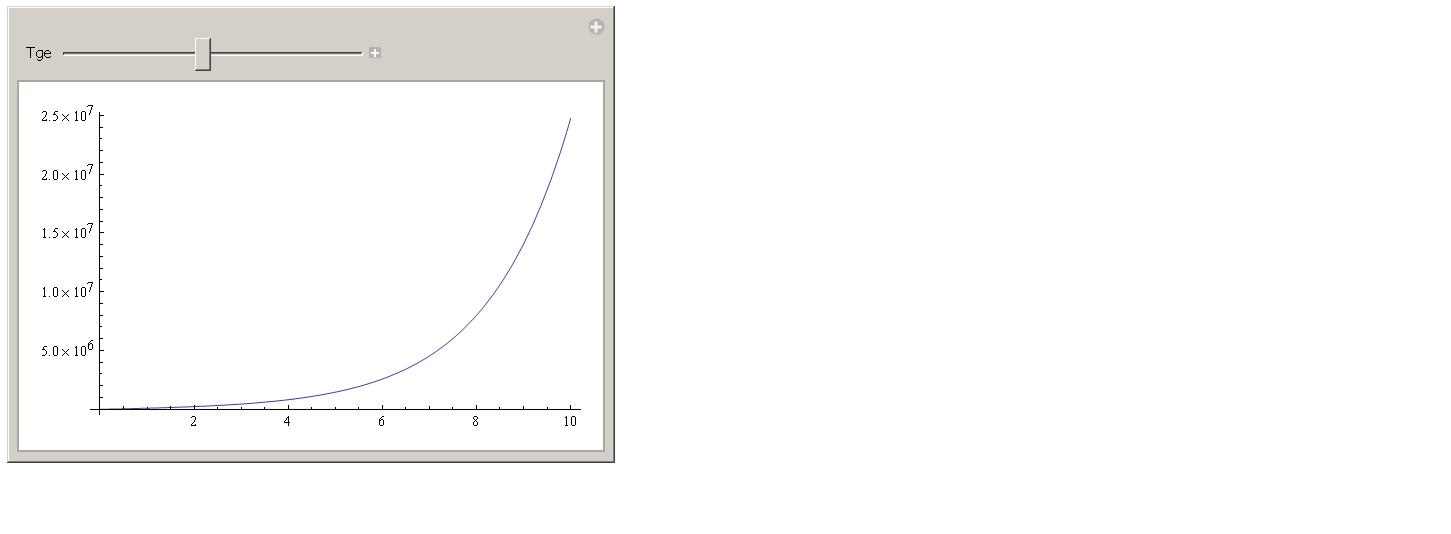As one can see, the left-hand part of eq1 very rapidly increases with Tc, if Tge is in the range of few tens. If this is OK with you, one can solve the equation numerically:

    Clear[Tge];
eq1 = (0.68 E^(-0.935 Tc) (-2.` + 2.` E^(0.5` Tc) + 
      E^(0.5` Tc + 0.935 Tge) (-2. + 2.` E^(1. Tc))))/(-2.3 + 
    2.3 E^(0.435 Tge)) == 0.66;
lst = Table[{Tge, FindRoot[eq1, {Tc, Tge}][[1, 2]]}, {Tge, 0.1, 10, 
    0.05}];
ListPlot[lst, AxesLabel -> {"Tge", "Tc"}]

You get the following plot: 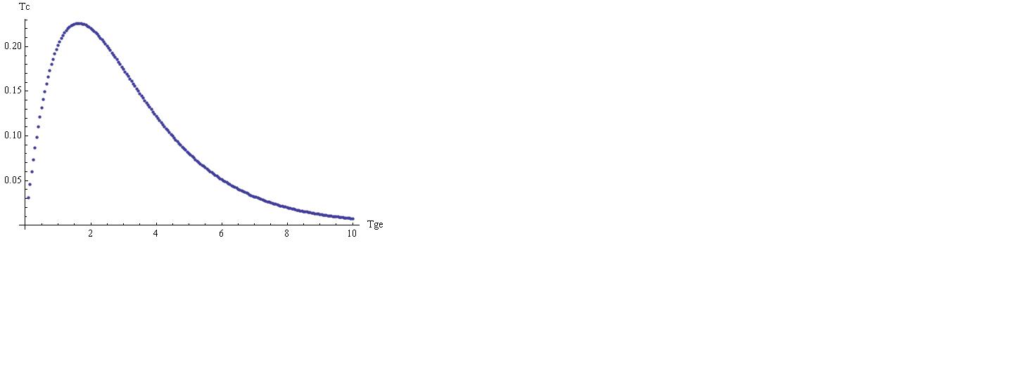Finally, if I would be at your place and need an analytic solution, I would fit it to some reasonable function. Like this, for example:

    Clear[a, b];
ff = FindFit[lst, a*x*Exp[-b*x], {a, b}, x];
Show[{
  ListPlot[lst, AxesLabel -> {"Tge", "Tc"}],
  Plot[a*x*Exp[-b*x] /. ff, {x, 0, 10}, PlotStyle -> Red]
  }]

You should see the following: 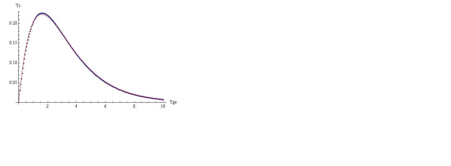The red line shows the fitting function. Have fun!