33
$\begingroup$

I'm a biologist and a newbie in Mathematica. I want to fit three data sets to a model consisting of four differential equations and 10 parameters. I want to find the parameters best fitting to my model. I have searched the forum and found several related examples. However, I could not find anything that matched my question.

Here are the details:

I have three time-series datasets: (xdata, ydata, zdata)

time = Quantity[{0, 3, 7, 11, 18, 25, 38, 59}, "seconds"];
tend = QuantityMagnitude[Last[time]];

xdata:

xdata = Quantity[{0, 0.223522, 0.0393934, 0.200991, 0.786874, 1, 
    0.265464, 0.106174}, "milligram"];
xfitdata = QuantityMagnitude[Transpose[{time, xdata}]];

ydata:

ydata = Quantity[{0, 0.143397, 0.615163, 0.628621, 0.53515, 0.519805, 
    0.757092, 1}, "milligram"];
yfitdata = QuantityMagnitude[Transpose[{time, ydata}]];

wdata:

wdata = Quantity[{0.0064948, 0.221541, 1, 0.434413, 0.732392, 
    0.458638, 0.1484432, 0.0294298}, "milligram"];
wfitdata = QuantityMagnitude[Transpose[{time, wdata}]];

I used ParametricNDSolve to solve the 4-DE model:

pfun = {x, y, z, w} /.  
  ParametricNDSolve[{x'[t] == 
     k1 - k10 x[t] w[t - 25] - k2 x[t] - k3 w[t] w[t], 
    y'[t] == -k8 y[t] + k10 x[t] w[t - 25] + k3 w[t] x[t], 
    z'[t] == k4 y[t] - k5 z[t], 
    w'[t] == (k6 x[t])/(y[t]^n + 1) - k7 w[t], x[t /; t <= 0] == 0.01,
     y[t /; t <= 0] == 0.01, z[t /; t <= 0] == 0.01, 
    w[t /; t <= 0] == 0.01}, {x, y, z, w}, {t, 0, tend}, {k1, k2, k3, 
    k4, k5, k6, k7, k8, n, k10}]

Then I used FindFit. But I don't know how to specify that xdata is supposed to be fitted to x[t], zdata to z[t] and wdata to w[t] via least-squares fit. For y[t], there are no time-series data, but the parameter (k8) for y[t] is supposed to be determined as well.

I have tried the following, which is apparently wrong:

fit = FindFit[xfitdata, 
  pfun[{k1, k2, k3, k4, k5, k6, k7, k8, n, k10}][
   t], {{k1, 0.0859}, {k2, 0.0125}, {k3, 0.8541}, {k4, 0.0185}, {k5, 
    0.1004}, {k6, 0.5002}, {k7, 0.0511}, {k8, 0.0334}, {n, 9}, {k10, 
    0.8017}}, t]

This is the error message:

FindFit::nrlnum: The function value {0. +<<1>>[0.],-0.223522+<<1>>,-0.0393934+<<1>>,-0.200991+<<1>>,-0.786874+<<1>>[{0.0859,0.0125,0.8541,0.0185,0.1004,0.5002,0.0511,0.0334,9.,0.8017}][18.],-1.+<<1>>[25.],-0.265464+<<1>>,-0.106174+<<1>>[59.]} is not a list of real numbers with dimensions {8} at {k1,k2,k3,k4,k5,k6,k7,k8,n,k10} = {0.0859,0.0125,0.8541,0.0185,0.1004,0.5002,0.0511,0.0334,9.,0.8017}. >>

I'm lost and I would really appreciate your help!

$\endgroup$
5
  • 2
    $\begingroup$ Am I correct that you are trying to fit about 20 data points to 4 equations with 10 parameters? I'm very interested in what you are modeling here. $\endgroup$ Commented Jul 12, 2013 at 12:43
  • 2
    $\begingroup$ @bobthechemist maybe it doesn't matter. After all, it's said that one can fit an elephant with five parameters...! $\endgroup$ Commented Jul 12, 2013 at 13:07
  • $\begingroup$ Also, is pfun even a function? Should it be pfun[{k1_,k2_…,k10_}]:= *definition* or something? I'm afraid I have to agree with the other comments that your task is almost impossible with the paucity of data and the number of parameters. (This would probably never survive a sensitivity analysis) But, I am interested in the general problem of fitting differential equation parameters to data sets... $\endgroup$
    – Eric Brown
    Commented Jul 12, 2013 at 13:26
  • 4
    $\begingroup$ @OleksandrR. And it's much easier if the elephant is inside a hat $\endgroup$ Commented Jul 12, 2013 at 14:04
  • 1
    $\begingroup$ @Stefanie could you please look over your question again and make sure the data and model are consistent? Initially you refer to the datasets as x, y, and z; then it becomes x, y, and w, and later x, z, and w. $\endgroup$ Commented Jul 13, 2013 at 17:27

2 Answers 2

32
$\begingroup$

Since the question isn't clear about which datasets are which and arguably has too many parameters, I'll use the example from here instead:

$$ \begin{array}{l} A+B\underset{k_2}{\overset{k_1}{\leftrightharpoons }}X \\ X+B\overset{k_3}{\longrightarrow }\text{products} \\ \end{array} \Bigg\} \Longrightarrow A+2B\longrightarrow \text{products} $$

We solve the system and generate some fake data:

sol = ParametricNDSolveValue[{
    a'[t] == -k1 a[t] b[t] + k2 x[t], a[0] == 1,
    b'[t] == -k1 a[t] b[t] + k2 x[t] - k3 b[t] x[t], b[0] == 1,
    x'[t] == k1 a[t] b[t] - k2 x[t] - k3 b[t] x[t], x[0] == 0
    }, {a, b, x}, {t, 0, 10}, {k1, k2, k3}
   ];

abscissae = Range[0., 10., 0.1];
ordinates = With[{k1 = 0.85, k2 = 0.15, k3 = 0.50},
   Through[sol[k1, k2, k3][abscissae], List]
  ];

data = ordinates + RandomVariate[NormalDistribution[0, 0.1^2], Dimensions[ordinates]];
ListLinePlot[data, DataRange -> {0, 10}, PlotRange -> All, AxesOrigin -> {0, 0}]

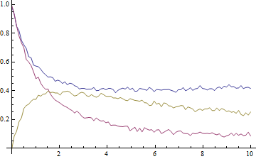
The data look like this, where blue is A, purple is B, and gold is X:

Plot of kinetic traces

The key to the exercise, of course, is the simultaneous fitting of all three datasets in order for the rate constants to be determined self-consistently. To achieve this we have to prepend to each point a number, i, that labels the dataset:

transformedData = {
    ConstantArray[Range@Length[ordinates], Length[abscissae]] // Transpose,
    ConstantArray[abscissae, Length[ordinates]],
    data
   } ~Flatten~ {{2, 3}, {1}};

We also need a model that returns the values for either A, B, or X depending on the value of i:

model[k1_, k2_, k3_][i_, t_] := 
  Through[sol[k1, k2, k3][t], List][[i]] /;
    And @@ NumericQ /@ {k1, k2, k3, i, t};

The fitting is now straightforward. Although it will help if reasonable initial values are given, this is not strictly necessary here:

fit = NonlinearModelFit[
   transformedData,
   model[k1, k2, k3][i, t],
   {k1, k2, k3}, {i, t}
  ];

Result of fitting

The result is correct. Worth noting, however, is that the off-diagonal elements of the correlation matrix are quite large:

fit["CorrelationMatrix"]
(* -> {{ 1.,        0.764364, -0.101037},
       { 0.764364,  1.,       -0.376295},
       {-0.101037, -0.376295,  1.      }} *)

Just to be sure of having directly addressed the question, I will note that the process does not change if we have less than the complete dataset available (although the parameters might be determined with reduced accuracy in this case). Typically it will be most difficult experimentally to measure the intermediate, so let's get rid of the dataset for X (i == 3) and try again:

reducedData = DeleteCases[transformedData, {3, __}];
fit2 = NonlinearModelFit[
   reducedData,
   model[k1, k2, k3][i, t],
   {k1, k2, k3}, {i, t}
  ];

The main consequence is that the error on $k_3$ is significantly larger:

Result of fitting without concentration data for X

This can be seen to be the result of greater correlation between $k_1$ and $k_3$ when fewer data are available for fitting:

fit2["CorrelationMatrix"]
(* -> {{ 1.,        0.7390200,  -0.1949590},
       { 0.7390200, 1.,          0.0435416},
       {-0.1949590, 0.0435416,   1.       }} *)

On the other hand, the correlation between $k_2$ and $k_3$ is greatly reduced, so that all of the rate constants are still sufficiently well determined and the overall result does not change substantially.

$\endgroup$
6
  • $\begingroup$ You have saved my day! Thank you so much for your answers @bobthechemist & Oleksandr R.! I have learned much from both answers! And sorry for the confusion as to the provided datasets! However, the main problem was how to fit differential equation parameters to multiple data sets. Now I know ... $\endgroup$
    – Stefanie
    Commented Jul 14, 2013 at 21:14
  • $\begingroup$ In evaluating the line defining "fit," I end up getting an error of (at t ~ 2.65) "step size is effectively zero; singularity or stiff system suspected," regardless of whether or not I input Method -> "StiffnessSwitching" in Mathematica 9.0.1. Has anyone else had this issue? I tried re-copying each section in a new notebook (as opposed to the within the NB example you linked to) to no avail. $\endgroup$
    – Ghersic
    Commented Jul 24, 2013 at 20:33
  • $\begingroup$ @Ghersic this message comes about due to NonlinearModelFit's usage (as trial values, in the process of fitting) of some combination of parameter values that make the system difficult to solve. It doesn't affect the result since the fit will pull the parameters toward their correct values and the error will disappear long before the fit converges. It can be avoided altogether if you specify initial guesses that are somewhat suitable for the system you're interested in solving, so that no attempts are made with wildly incorrect parameter values. $\endgroup$ Commented Jul 26, 2013 at 14:11
  • $\begingroup$ @OleksandrR. Ah, alright; I had noticed your comment on this but didn't think to apply it. Thank you again, I really appreciate it. $\endgroup$
    – Ghersic
    Commented Jul 28, 2013 at 15:41
  • $\begingroup$ I'm not mistaken in thinking that, for a properly constructed system, this specification of reasonable initial parameters occurs in the definition of "ordinates," am I? I don't see where but I feel there might be some other area where I should do this as well. $\endgroup$
    – Ghersic
    Commented Aug 11, 2013 at 0:34
21
$\begingroup$

Note Added in proof

Oleksander's answer provides a better fit to the data than my solution below and circumvents the reiteration-and-solving-individually problem I describe below.

This is not an answer to your question specifically, but rather is one method to use ParametricNDSolve to fit experimental data.

Defining the problem

$\require{mhchem}$ Differential equations come in to play in chemical kinetics, most notably in determining the rates of reactions. Consider the following reaction $\ce{A -> B + C}$. To my knowledge, the set of equations that describe the differential rate laws for the three components of this system cannot be solved analytically. Let's say that we have collected a set of concentration vs. time data for each of the three species A, B, and C and would like to fit the data to this chemical equation. First, I will make some data, noting that if the rate constant for the reverse reaction is k then the rate of the forward reaction can be given by K x k where K is the equilibrium constant for the chemical equation.

tdata = NDSolve[{a'[t] == -b'[t] == -c'[t] == -k K a[t] + k b[t] c[t],
     a[0] == a0, b[0] == b0, c[0] == c0} /. {K -> 3, k -> 1, 
    a0 -> 0.5, b0 -> 0.4, c0 -> 0.1}, {a[t], b[t], c[t]}, {t, 0, 1}]
edata = Flatten[
   Table[{t, RandomReal[{0.98, 1.02}] a[t], 
      RandomReal[{0.98, 1.02}] b[t], 
      RandomReal[{0.98, 1.02}] c[t]} /. tdata, {t, 0, 1, 0.05}], 1];

Here, I've chosen the answers to be k = 1, K = 3, and the initial concentrations of A, B, and C to be 0.5, 0.4, and 0.1, respectively.
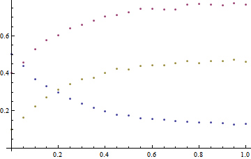
experimental data to fit

Solving the problem

We start by using ParametricNDSolve to generate the interpolation functions, and generate a plot just to make sure we are on the right track.

sol = ParametricNDSolve[{a'[t] == -b'[t] == -c'[t] == -k K a[t] + 
     k b[t] c[t], a[0] == a0, b[0] == b0, c[0] == c0}, {a, b, c}, {t, 
   0, 1}, {k, K, a0, b0, c0}];
a1 = a[1, 3, 0.5, 0.4, 0.1] /. sol;
b1 = b[1, 3, 0.5, 0.4, 0.1] /. sol;
c1 = c[1, 3, 0.5, 0.4, 0.1] /. sol;
Plot[Evaluate@{a1[t], b1[t], c1[t]}, {t, 0, 1}]
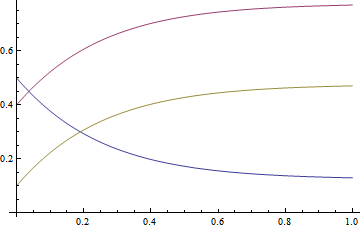
Interpolated functions

Using NonlinearModelFit with ParametricNDsolve solutions

The solutions from ParametricNDSolve can be used directly in the NonlinearModelFit function, providing results that seem to provide a decent fit. Note that fitting the concentration data for B and C threw errors (more on that below).

nlma = NonlinearModelFit[edata[[All, {1, 2}]], 
  a[k, K, a0, b0, c0][t] /. sol, {k, K, a0, b0, c0}, t]
nlmb = NonlinearModelFit[edata[[All, {1, 3}]], 
  b[k, K, a0, b0, c0][t] /. sol, {k, K, a0, b0, c0}, t]
nlmc = NonlinearModelFit[edata[[All, {1, 4}]], 
  c[k, K, a0, b0, c0][t] /. sol, {k, K, a0, b0, c0}, t]

The results look pretty good, however the parameters are actually meaningless:
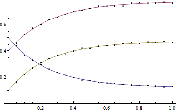
bad results

bad results table

Adding constraints

This problem can be improved by adding constraints to the NonlinearModelFit

nlma2 = NonlinearModelFit[
  edata[[All, {1, 2}]], {a[k, K, a0, b0, c0][t] /. sol2, k > 0, K > 0,
    0 < a0 < 1, 0 < b0 < 1, 0 < c0 < 1}, {k, K, a0, b0, c0}, t]
nlmb2 = NonlinearModelFit[
  edata[[All, {1, 3}]], {b[k, K, a0, b0, c0][t] /. sol2, k > 0, K > 0,
    0 < a0 < 1, 0 < b0 < 1, 0 < c0 < 1}, {k, K, a0, b0, c0}, t]
nlmc2 = NonlinearModelFit[
  edata[[All, {1, 4}]], {c[k, K, a0, b0, c0][t] /. sol2, k > 0, K > 0,
    0 < a0 < 1, 0 < b0 < 1, 0 < c0 < 1}, {k, K, a0, b0, c0}, t]

better fit

The fit is better, but still not great, and it is important to note that the data sets for each individual concentration give varying optimal parameters. I'm a fan of the brute force and ignorance approach, and one way to address the problem with the parameters is to take the Mean and StandardDeviation of the "optimal" parameters and use these as new constraints.

(* New stuff *)
mean = Mean[{k, K, a0, b0, c0} /. #["BestFitParameters"] & /@ {nlma2, 
    nlmb2, nlmc2}]
sd = StandardDeviation[{k, K, a0, b0, c0} /. #[
      "BestFitParameters"] & /@ {nlma2, nlmb2, nlmc2}]
const = MapThread[{#1 - #2 < #3 < #1 + #2} &, {mean, 
   sd, {k, K, a0, b0, c0}}]
(* old stuff *)
nlma3 = NonlinearModelFit[
  edata[[All, {1, 2}]], {a[k, K, a0, b0, c0][t] /. sol2, const}, {k, 
   K, a0, b0, c0}, t]
nlmb3 = NonlinearModelFit[
  edata[[All, {1, 3}]], {b[k, K, a0, b0, c0][t] /. sol2, const}, {k, 
   K, a0, b0, c0}, t]
nlmc3 = NonlinearModelFit[
  edata[[All, {1, 4}]], {c[k, K, a0, b0, c0][t] /. sol2, const}, {k, 
   K, a0, b0, c0}, t]
TableForm[{k, K, a0, b0, c0} /. #["BestFitParameters"] & /@ {nlma3, 
   nlmb3, nlmc3}, 
 TableHeadings -> {{"a", "b", "c"}, {"k(1)", "K(3)", "a0(0.5)", 
    "b0(0.4)", "c0(0.1)"}}]

even better results

We are now starting to get agreement between the three sets of data. After repeating this loop approximately a dozen times, the results start to settle:

Best fit

Conclusion

We can see that some of the best fit parameters are reasonably close to the actual values (concentrations of A and B) what might be considered the important values (k and K) have appreciable, but possibly acceptable errors (on the order of 20 to 30%). I presume, although have not tested, that part of the problem lies in redefining the constraints for concentration of C, which from the first iteration did not contain the true value. The conclusion to draw from this exercise is that a complex model (and this is not a terribly complex model) will give you a fit of the data, but you need to know something about the reality of the parameters before you can actually trust the fit. Maybe Mathematica version 10 will provide that insight, but as of now, we must use our own brains to determine the value of a fit.

$\endgroup$
5
  • $\begingroup$ I think this is not the right way to self-consistency, since simultaneous fitting gives much better estimates for the same system. Several of the parameters are very strongly correlated, which is difficult to assess in an iterative scheme and potentially adds to the difficulties inherent in it. $\endgroup$ Commented Jul 14, 2013 at 1:57
  • $\begingroup$ @oleksandr I agree - due to my inability to spell abscissae it took me much longer to reproduce your results on my system. I've noted your solution is superior to mine at the top of my answer. $\endgroup$ Commented Jul 14, 2013 at 12:11
  • $\begingroup$ Thanks a lot @bobthechemist! As I have written below @Oleksandr R.'s answer, your answer helps me a lot! $\endgroup$
    – Stefanie
    Commented Jul 14, 2013 at 21:21
  • $\begingroup$ Dear bob, hopefully you now have an idea on how to make MathJax bend to any of your chemical whims. :) Best regards. $\endgroup$ Commented May 26, 2015 at 15:24
  • $\begingroup$ @J. M. I'll bet a nickel that the chem tag for MathJax wasn't working at the time I wrote this answer, although since my comment above indicates I had spelling issues back then, it's possible I was spelling "ce" incorrectly as well. $\endgroup$ Commented May 27, 2015 at 1:12

Your Answer

By clicking “Post Your Answer”, you agree to our terms of service and acknowledge you have read our privacy policy.

Not the answer you're looking for? Browse other questions tagged or ask your own question.