Why does NDSolve fail to converge when solving for Sadowsky ribbon with nonzero θ?

Question

I am working with the control equations of a Sadowsky ribbon, where the basic equations eqs and boundary conditions bc0 and bc1 are derived from the Kirchhoff rod theory, and have been validated. These equations are relatively straightforward, but the Sadowsky ribbon has a nonlinear constitutive relation, which is given in the eqsadd set, and the corresponding boundary conditions given in the bc0add set.

\[Theta] = 0; init = {9, 0, 0, 0, 0, -50, 9, 0}; 
eqs = {x'[s] == d3x[s], y'[s] == d3y[s], z'[s] == d3z[s], n1'[s] == n2[s]*k3[s], n2'[s] == n3[s]*k1[s] - n1[s]*k3[s], n3'[s] == -n2[s]*k1[s], d3x'[s] == -k1[s]*d2x[s], d3y'[s] == -k1[s]*d2y[s], d3z'[s] == -k1[s]*d2z[s], M1'[s] == M2[s]*k3[s] + n2[s], M2'[s] == M3[s]*k1[s] - M1[s]*k3[s] - n1[s], M3'[s] == -M2[s]*k1[s],d1x'[s] == k3[s]*d2x[s], d2x'[s] == k1[s]*d3x[s] - k3[s]*d1x[s], d1y'[s] == k3[s]*d2y[s], d2y'[s] == k1[s]*d3y[s] - k3[s]*d1y[s], d1z'[s] == k3[s]*d2z[s], d2z'[s] == k1[s]*d3z[s] - k3[s]*d1z[s]}; 
bc0 = {x[0] == 0, y[0] == 0, z[0] == 0, d1x[0] == 0, d1y[0] == 0, d1z[0] == 1, d2x[0] == 0, d2y[0] == -1, d2z[0] == 0, d3x[0] == 1, d3y[0] == 0, d3z[0] == 0}; 
bc1 = {x[1] == 0.5, y[1] == 0, z[1] == 0, Cos[\[Theta]]  d1y[1] + d1z[1]  Sin[\[Theta]] == 0, d2x[1] == 0, Cos[\[Theta]]  d3z[1] - d3y[1]  Sin[\[Theta]] == 0}; 
var = {x, y, z, d1x, d1y, d1z, d2x, d2y, d2z, d3x, d3y, d3z, M1, M2, M3, n1, n2, n3, k1, k3}; 
eqsadd = {k1'[s] == (k1[s]^4  (M2[s]  k3[s]  (k1[s]^2 + k3[s]^2) + n2[s]  (k1[s]^2 + 3  k3[s]^2)))/(((k1[s]^2 + k3[s]^2)^3)), k3'[s] == (k1[s]^3  (4 n2[s]  k3[s]^3 + M2[s]  (-k1[s]^4 + k3[s]^4)))/((2  (k1[s]^2 + k3[s]^2)^3))}; 
bc0add = {M1[0]*k1[0]^3 == k1[0]^4 - k3[0]^4, M3[0]*k1[0]^2 == 2 (k1[0]^2 +k3[0]^2)*k3[0]}; 
sol = NDSolve[Join[eqs, bc0, bc1, eqsadd, bc0add], var, {s, 0, 1}, Method -> {"Shooting", "StartingInitialConditions" -> {M1[0] == init[[1]], M2[0] == init[[2]], M3[0] == init[[3]], n1[0] == init[[4]], n2[0] == init[[5]], n3[0] == init[[6]], k1[0] == init[[7]], k3[0] == init[[8]]}, MaxIterations -> 10000}]

I have also supplied the init set, which serves as the initial guess when applying the shooting method. The results appear quite good. However, the issue arises when I attempt to solve the system with θ ≠ 0 (where θ represents an angle parameter). Even if θ is small, Mathematica fails to achieve a convergent solution. I have experimented with multiple solvers, but the problem still persists.

Is there a specific reason why Mathematica has difficulty converging in this situation? Are there any techniques or strategies I can use to help resolve this issue and obtain a solution?

Any insights would be greatly appreciated. Thank you!

Answer 1

Solution for $\theta=\pi/3$ can be computed in 3 step. On the first step we use the Euler wavelets collocation method and NMinimize to compute initial data for FindRoot as follows (please, note that we use algebraic equations for M1[s], M3[s] instead of differential equations for k1[s], k3[s])

eqs = {x'[s] == d3x[s], y'[s] == d3y[s], z'[s] == d3z[s], 
  n1'[s] == n2[s]*k3[s], n2'[s] == n3[s]*k1[s] - n1[s]*k3[s], 
  n3'[s] == -n2[s]*k1[s], d3x'[s] == -k1[s]*d2x[s], 
  d3y'[s] == -k1[s]*d2y[s], d3z'[s] == -k1[s]*d2z[s], 
  M1'[s] == M2[s]*k3[s] + n2[s], 
  M2'[s] == M3[s]*k1[s] - M1[s]*k3[s] - n1[s], M3'[s] == -M2[s]*k1[s],
   d1x'[s] == k3[s]*d2x[s], d2x'[s] == k1[s]*d3x[s] - k3[s]*d1x[s], 
  d1y'[s] == k3[s]*d2y[s], d2y'[s] == k1[s]*d3y[s] - k3[s]*d1y[s], 
  d1z'[s] == k3[s]*d2z[s], d2z'[s] == k1[s]*d3z[s] - k3[s]*d1z[s], 
  M1[s] == k1[s] (1 - k3[s]^4/k1[s]^4), 
  M3[s] == 2 (1 + k3[s]^2/k1[s]^2)*k3[s]}; bc0 = {x[0] == 0, 
  y[0] == 0, z[0] == 0, d1x[0] == 0, d1y[0] == 0, d1z[0] == 1, 
  d2x[0] == 0, d2y[0] == -1, d2z[0] == 0, d3x[0] == 1, d3y[0] == 0, 
  d3z[0] == 0};
bc1 = {x[1] == 0.5, y[1] == 0, z[1] == 0, 
  Cos[t] d1y[1] + d1z[1] Sin[t] == 0, d2x[1] == 0, 
  Cos[t] d3z[1] - d3y[1] Sin[t] == 0}; var = {x, y, z, d1x, d1y, d1z, 
  d2x, d2y, d2z, d3x, d3y, d3z, M1, M2, M3, n1, n2, n3, k1, 
  k3}; init = {9, 0, 0, 0, 0, -50, 9, 0}; ini = {M1[0] == init[[1]], 
  M2[0] == init[[2]], M3[0] == init[[3]], n1[0] == init[[4]], 
  n2[0] == init[[5]], n3[0] == init[[6]], k1[0] == init[[7]], 
  k3[0] == init[[8]]}; bc0add = {M1[0] == k1[0] (1 - k3[0]^4/k1[0]^4),
   M3[0] == 2 (1 + k3[0]^2/k1[0]^2)*k3[0]};

bc = Join[bc0, bc0add, bc1];

UE[m_, t_] := EulerE[m, t];
psi[k_, n_, m_, t_] := 
  Piecewise[{{2^(k/2) UE[m, 2^k t - 2 n + 1], (n - 1)/2^(k - 1) <= t <
       n/2^(k - 1)}, {0, True}}];
PsiE[k_, M_, t_] := 
 Flatten[Table[psi[k, n, m, t], {n, 1, 2^(k - 1)}, {m, 0, M - 1}]]
k0 = 2; M0 = 3; With[{k = k0, M = M0}, 
 nn = Length[Flatten[Table[1, {n, 1, 2^(k - 1)}, {m, 0, M - 1}]]]];
dx = 1/(nn); xl = Table[l*dx, {l, 0, nn}]; scol = 
 Table[(xl[[l - 1]] + xl[[l]])/2, {l, 2, nn + 1}]; Psijk = 
 With[{k = k0, M = M0}, PsiE[k, M, t1]]; Int1 = 
 With[{k = k0, M = M0}, Integrate[PsiE[k, M, t1], t1]];
Int2 = Integrate[Int1, t1];
Psi[y_] := Psijk /. t1 -> y; 
int1[y_] := Int1 /. t1 -> y; V = Array[vv, {nn, Length[var]}];


vart = Table[var[[i]]@s, {i, Length[var]}]; dvart = D[vart, s]; U = 
 Array[uu, {Length[var]}]; rule = 
 Flatten[Table[{vart[[i]] -> V[[All, i]] . int1[s] + U[[i]], 
    dvart[[i]] -> V[[All, i]] . Psi[s]}, {i, Length[var]}], 1];
eqn = (eqs[[All, 1]] - eqs[[All, 2]]) /. rule;
vart0 = vart /. s -> 0; vart1 = vart /. s -> 1; rulebc = 
 Flatten[Table[{vart0[[i]] -> V[[All, i]] . int1[0] + U[[i]], 
    vart1[[i]] -> V[[All, i]] . int1[1] + U[[i]]}, {i, Length[var]}], 
  1]; bcn = (bc[[All, 1]] - bc[[All, 2]]) /. rulebc;

eqAll = Join[Flatten@Table[eqn, {s, scol}], 
  bcn /. t -> Pi/3]; varAll = Join[Flatten@V, U];

em = Flatten@Table[eqn, {s, scol}]; bt = bcn /. t -> Pi/3;
sol1 = NMinimize[{em . em, Table[bt[[i]] == 0, {i, Length[bt]}]}, 
  varAll]; 

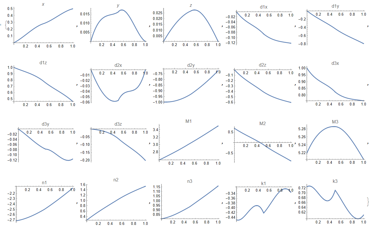
As results we have first initial state

Table[Plot[V[[All, i]] . int1[s] + U[[i]] /. sol1[[2]], {s, 0, 1}, 
  PlotLabel -> var[[i]]], {i, Length[var]}]

On the second step we polish initial solution sol1 with FindRoot as follows

sol = FindRoot[Table[eqAll[[i]] == 0, {i, Length[eqAll]}], 
  Table[{varAll[[i]], varAll[[i]] /. sol1[[2]]}, {i, Length[varAll]}],
   MaxIterations -> 1000];

As result we have initial data for NDSolve

inif = 
 Table[V[[All, i]] . int1[0] + U[[i]] /. sol, {i, Length[var]}]

Out[]= {0., 0., 0., 0., 0., 1., 0., -1., 0., 1., 0., 0., 10.0989, \
-85.8467, 11.9765, -194.962, 28.5576, 455.311, -0.494493, 1.06396}

Finally, we use inif as initial data for NDSolve as

eqs0 = {x'[s] == d3x[s], y'[s] == d3y[s], z'[s] == d3z[s], 
   n1'[s] == n2[s]*k3[s], n2'[s] == n3[s]*k1[s] - n1[s]*k3[s], 
   n3'[s] == -n2[s]*k1[s], d3x'[s] == -k1[s]*d2x[s], 
   d3y'[s] == -k1[s]*d2y[s], d3z'[s] == -k1[s]*d2z[s], 
   M1'[s] == M2[s]*k3[s] + n2[s], 
   M2'[s] == M3[s]*k1[s] - M1[s]*k3[s] - n1[s], 
   M3'[s] == -M2[s]*k1[s], d1x'[s] == k3[s]*d2x[s], 
   d2x'[s] == k1[s]*d3x[s] - k3[s]*d1x[s], d1y'[s] == k3[s]*d2y[s], 
   d2y'[s] == k1[s]*d3y[s] - k3[s]*d1y[s], d1z'[s] == k3[s]*d2z[s], 
   d2z'[s] == k1[s]*d3z[s] - k3[s]*d1z[s], 
   k1'[s] == (k1[s]^4 (M2[s] k3[s] (k1[s]^2 + k3[s]^2) + 
         n2[s] (k1[s]^2 + 3 k3[s]^2)))/(((k1[s]^2 + k3[s]^2)^3)), 
   k3'[s] == (k1[s]^3 (4 n2[s] k3[s]^3 + 
         M2[s] (-k1[s]^4 + k3[s]^4)))/((2 (k1[s]^2 + k3[s]^2)^3))};

sol2 = NDSolve[{eqs0, bc} /. t -> Pi/3, var, {s, 0, 1}, 
  Method -> {"Shooting", 
    "StartingInitialConditions" -> Thread[vart0 == inif]}];

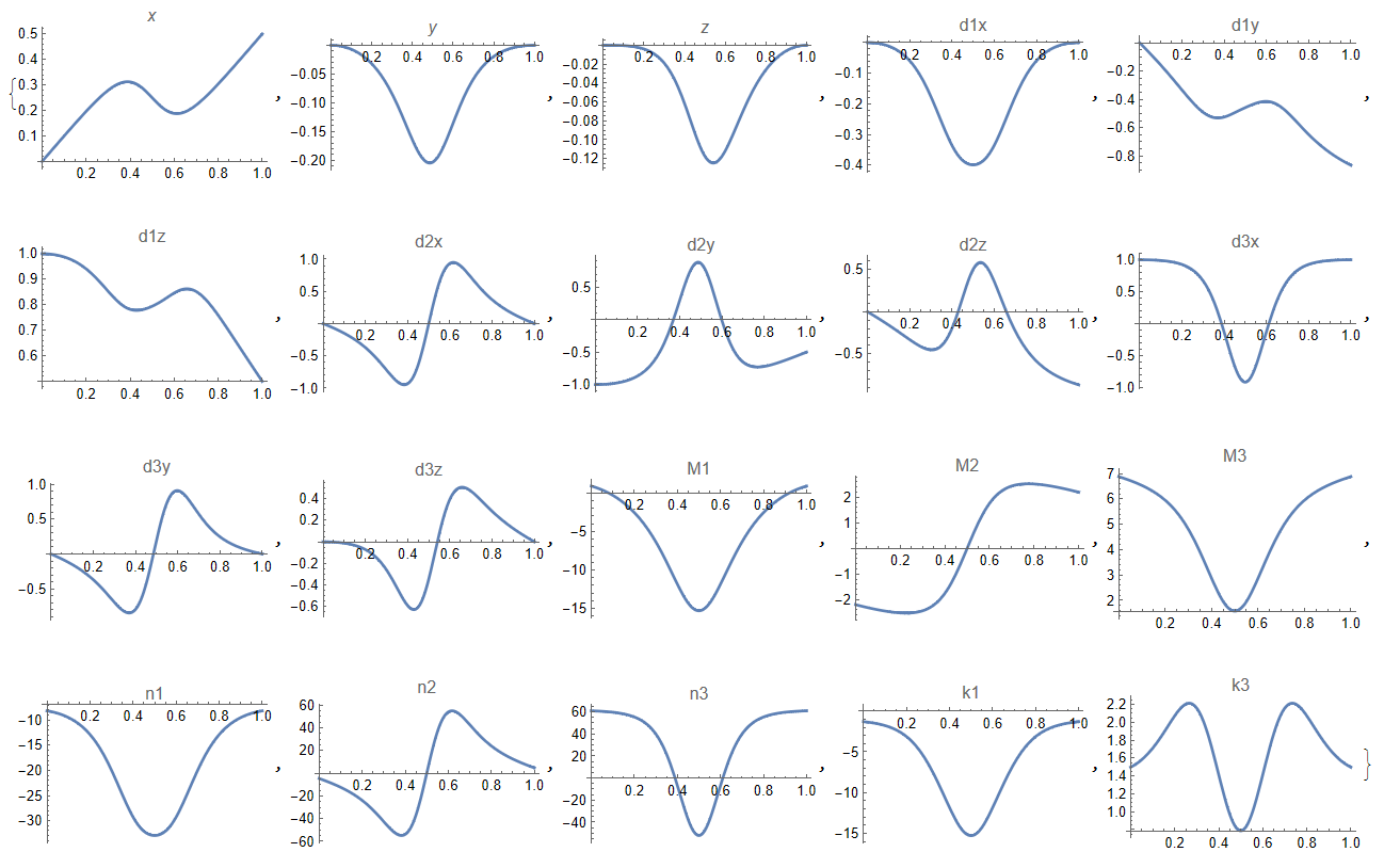
Visualization

Table[Plot[vart[[i]] /. sol2[[1]], {s, 0, 1}, 
  PlotLabel -> var[[i]]], {i, Length[var]}]

Answer 2

This answer provides solutions over a wide range of θ for the system of equations given in the question. Edited to extend range of θ to {0, 3/2 Pi}.

To begin, multiple solutions exist for θ = 0. To illustrate, it is convenient to use the code in the question but with the first line, which defines θ and init, omitted and the last line replaced by

init = {9, 0, 0, 0, 0, -50, 9, 0};
sol = Flatten@NDSolve[{eqs, bc0, bc1, eqsadd, bc0add} /. θ -> 0, 
    var, {s, 0, 1}, Method -> {"Shooting", "StartingInitialConditions" -> 
    Thread[Through[var[[13 ;; 20]]@0] == init]}];
Chop[Through[var[[13 ;;]]@0] /. sol]
(* {1.20259, 0, 0, 0, -0.0000126724, 62.7307, 1.20259, 0} *)

which is, I presume, the same answer obtained by the OP. In contrast, replacing this init by init = {9, 0, 0, 0, 0, 50, 9, 0}; yields

(* {3.5362, 0, 0, 0, 40.5173, 138.423, 3.5362, 0} *)

And, replacing it by init = {1, 0, 0, 0, 0, 50, 1, 0}; yields

(* {1.20259, 0, 0, 0, -0.0000126724, 62.7307, 1.20259, 0} *)

Experimentation shows that the first two init arrays produce solutions only for θ slightly larger than zero, and for larger values NDSolve fails to converge. (The question also makes this observation for the first init array.) In contrast, the third init array yields solutions for θ as large as 1.2. In particular,

init = {1, 0, 0, 0, 0, 50, 1, 0};
sol = Flatten@NDSolve[{eqs, bc0, bc1, eqsadd, bc0add} /. θ -> Pi/3, 
    var, {s, 0, 1}, Method -> {"Shooting", "StartingInitialConditions" -> 
    Thread[Through[var[[13 ;; 20]]@0] == init]}];
Chop[Through[var[[13 ;;]]@0] /. sol]
(* {-0.895113, 2.19402, 6.87672, 8.13244, 4.69525, 60.9908, 1.31501, 1.49727} *)

produces the same answer obtained by Alex Trounev, including his second set of plots. Solutions for θ -> Pi/4 and θ -> Pi/8 can be obtained in the same way:

{0.3292, 1.43142, 4.41963, 4.42162, 1.83149, 61.5116, 1.27868, 1.18698}

and

{1.09532, 0.544718, 1.75664, 1.25762, 0.25016, 62.3213, 1.21008, 0.67152}

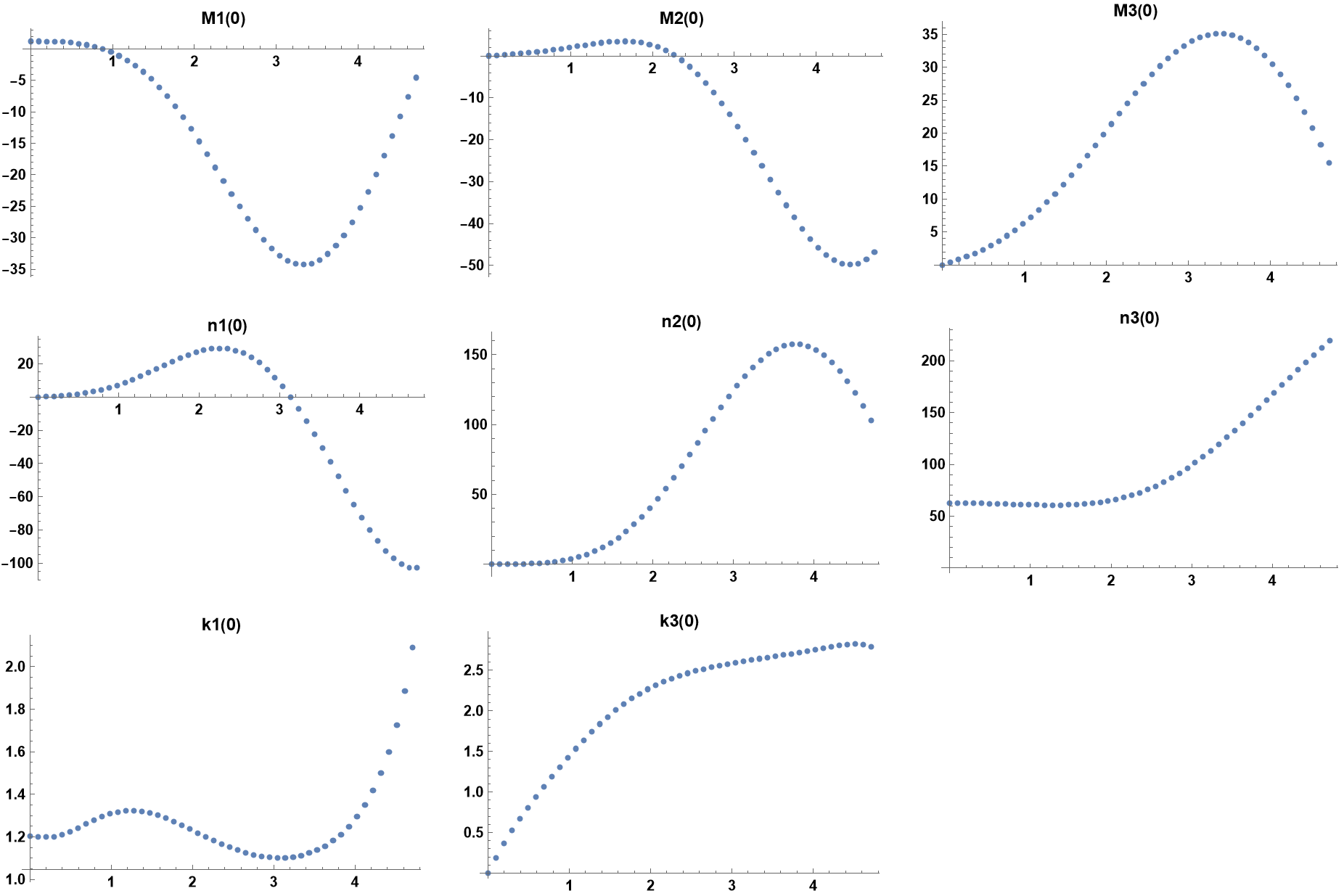
Solutions over a range of θ can be obtained with

init = {1, 0, 0, 0, 0, 50, 1, 0};
sol = Flatten@NDSolve[{eqs, bc0, bc1, eqsadd, bc0add} /. θ -> Pi/3, 
    var, {s, 0, 1}, Method -> {"Shooting", "StartingInitialConditions" -> 
    Thread[Through[var[[13 ;; 20]]@0] == init]}];
Chop[Through[var[[13 ;;]]@0] /. sol];

v0 = Transpose@Chop@FoldList[Flatten@NDSolveValue[{eqs, bc0, bc1, eqsadd, 
    bc0add} /. θ -> #2, Through[var[[13 ;;]]@0], {s, 0, 1}, 
    Method -> {"Shooting", "StartingInitialConditions" -> 
    Thread[Through[var[[13 ;; 20]]@0] == #1]}] &, %, Range[Pi/32, 3 Pi/2, Pi/32]];

Table[ListPlot[v0[[i]], DataRange -> {0, 3 Pi/2}, PlotRange -> All, 
    PlotLabel -> var[[12 + i]]@0, LabelStyle -> {Black, Bold, 10}], {i, 1, 8}];
GraphicsGrid[{%[[;; 3]], %[[4 ;; 6]], %[[7 ;;]]}, ImageSize -> Full]

Incidentally, I accidently found another solution for θ -> 15 Pi/32 with

(* {-1.32012, 46.399, -5.07669, 66.5504, 6.29148, 76.6438, 0.734378, -0.949765} *)

This suggests that there are multiple solutions for many values of θ.