I cant solve the following differential equation $$\frac{1}{x}\frac {d}{dx}\left(x\frac{df}{dx}\right)+\left( 1-\frac{1}{x^2}\right)f-f^3=0$$ with the boundary conditions $f(0)=0$ and $f(\infty)=1$. The second boundary condition causes a lot of problems. Can anyone help me please? This problem took a lot of my time. I tried to solve it with NDsolve but i didnt succed. PS: I have Mathematica12.1
-
$\begingroup$ does this ode have a name? i.e is it known in some field? $\endgroup$– NasserCommented Jun 28 at 11:35
-
$\begingroup$ Yes, it has a physical background. It is the radial density of a vortex in a superfluid. $\endgroup$– ClaraCommented Jun 28 at 12:05
-
2$\begingroup$ People here generally like users to post code as copyable Mathematica code as well as images or TeX, so they can copy-paste it. It makes it convenient for them and more likely you will get someone to help you. You may find the meta Q&A, How to copy code from Mathematica so it looks good on this site, helpful $\endgroup$– Michael E2Commented Jun 28 at 13:45
2 Answers
You can't solve with BC at infinity numerically. Since this BVP, you can try shooting method.
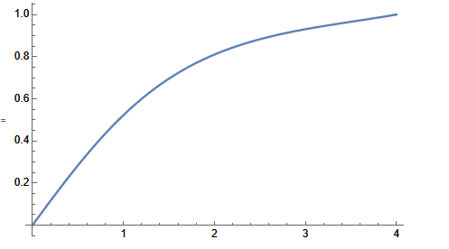
Best I could make run to is up to $x=4$
ode=1/x*D[x*f'[x],x]+(1-1/x^2)*f[x]-f[x]^3==0
k=4;
bc={f[$MachineEpsilon]==0,f[k]==1}

sol=NDSolve[{ode,bc},f,{x,$MachineEpsilon,k},
     Method->{"Shooting",
       "StartingInitialConditions"->{f[$MachineEpsilon]==0,f'[$MachineEpsilon]==1}},
        WorkingPrecision->40
 ]
Plot[Evaluate[f[x]/.sol],{x,0,k}]
There might be more tunning options to make it integrate to larger values.
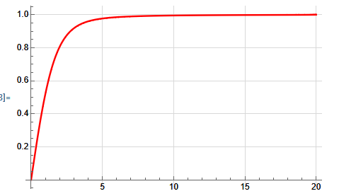
Thanks to comment below by Mariusz Iwaniuk, using f'[$MachineEpsilon]==Rationalize[1.166378991720675,0] makes it go to $x=20$.
sol = NDSolve[{ode, bc}, f, {x, $MachineEpsilon, k},
  Method -> {"Shooting",
    "StartingInitialConditions" -> {f[$MachineEpsilon] == 0,
      f'[$MachineEpsilon] == Rationalize[1.166378991720675, 0]}},
  WorkingPrecision -> 40]

 Plot[Evaluate[f[x] /. sol], {x, 0, k}, AxesOrigin -> {0, 0},
 PlotStyle -> Red, GridLines -> Automatic,
 GridLinesStyle -> LightGray]
-
1$\begingroup$ Thank you very much for that answer, but 4 seems very small in comparison to $\infty$ :D Is there maybe another way to set $\infty >10$ at least? This should be fine for what i need. $\endgroup$– ClaraCommented Jun 28 at 12:04
-
2$\begingroup$ Using Trial and Error and
Method -> {"Shooting", "StartingInitialConditions" -> {f[$MachineEpsilon] == 0, f'[$MachineEpsilon] == Rationalize[1.166378991720675, 0]}}` we can reach it fork=20. $\endgroup$ Commented Jun 28 at 14:52 -
$\begingroup$ Thank you very much for this answer. Helps a lot :) $\endgroup$– ClaraCommented Jun 30 at 6:53
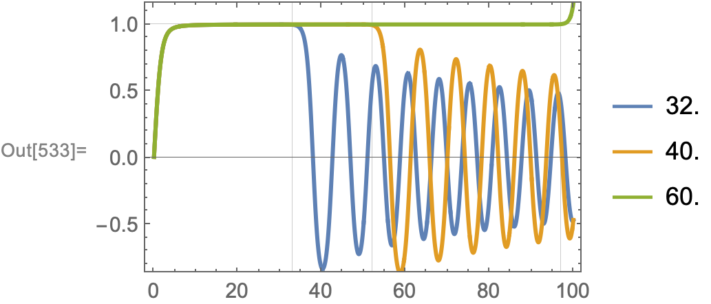
Use asymptotic expansion at $x=0$ of linearization of the ODE (the nonlinear term vanishes to high order there) to help get NDSolve started. Then used Brent's method to figure out initial conditions that solve the BVP using FindRoot[]. The working precision needs to be increased the further one wants to prolong the solution, which cannot be done by the built-in shooting method. Either you have to work with high precision all the way through, or do it manually. The NDSolve calls take a few seconds each. Consequently FindRoot takes a few minutes, since sometimes it takes more than one hundred iterations.
ode = 1/x*D[x*y'[x], x] + (1 - 1/x^2)*y[x] - y[x]^3 == 0 //
   MultiplySides[#, x^2] & // Simplify[#, x != 0] &
(*
x^2 y[x]^3 == (-1 + x^2) y[x] +
  x (Derivative[1][y][x] + x (y^\[Prime]\[Prime])[x])
*)

(* zero out nonlinear term *)
DSolveValue[{0 x^2  y[x]^3 == (-1 + x^2) y[x] +
    x (Derivative[1][y][x] + x (y^\[Prime]\[Prime])[x]), y[0] == 0},
 y[x], x]
(*
BesselJ[1, x]  C[1]
*)

uode = ode /. y -> Function[x, BesselJ[1, x]  u[x]] //
  FullSimplify[#, x > 0] &;

uasym // ClearAll;
uasym[x_, yp_] =
 AsymptoticDSolveValue[{uode, u[0] == 2 yp}, u[x], {x, 0, 10}]
yasym[x_, yp_] = BesselJ[1, x] uasym[x, yp];
uasym[0.01, yp]
uasym[0.001, yp]
(*
2 yp + (x^4 yp^3)/12 - (x^6 yp^3)/144 + (
 x^10 (-3 yp^3 - 136 yp^5))/230400 + (x^8 (11 yp^3 + 72 yp^5))/23040

2 yp + 8.33326*10^-10 yp^3 + 4.34028*10^-26 (-3 yp^3 - 136 yp^5) +
 4.34028*10^-21 (11 yp^3 + 72 yp^5)

2 yp + 8.33333*10^-14 yp^3 + 4.34028*10^-36 (-3 yp^3 - 136 yp^5) +
 4.34028*10^-29 (11 yp^3 + 72 yp^5)
*)
obj // ClearAll;
mem : obj[yp_?NumericQ, {x0_, xmax_}, wp_] :=
  mem = Block[{$MinPrecision = wp},
    ysol =
     Quiet@NDSolveValue[{ode, y[x0] == yasym[x0, yp],
        y'[x0] == D[yasym[x, yp], x] /. x -> x0}
       , y, {x, x0, xmax}, WorkingPrecision -> wp,
       Method -> {"Extrapolation", Method -> "LinearlyImplicitEuler"}];
    Quiet@ysol[xmax]
    ];

(* shoot for yp0 *)
With[{prec = 32},
 Inactive[FindRoot][obj[yp, {1/100, 100}, prec] == 1
  , {yp, 0.58, 0.59}
  , Method -> "Brent", WorkingPrecision -> prec]
 ]
yp0 = % // Activate
ysol0 = ysol;
(*
FindRoot::cvmit: Failed to converge to the requested accuracy or precision within 100 iterations.

{yp -> 0.58318949586032935129314612539441}
*)

(* shoot for yp1 *)
With[{prec = 40},
 Inactive[FindRoot][obj[yp, {1/100, 100}, prec] == 1
  , {yp, yp (1 - 10^(-Precision[yp0]/6)) /. yp0,
   yp (1 + 10^(-Precision[yp0]/6)) /. yp0}
  , Method -> "Brent", WorkingPrecision -> prec,
  MaxIterations -> 150]
 ]
yp1 = % // Activate
ysol1 = ysol;
(*
FindRoot::cvmit: Failed to converge to the requested accuracy or precision within 150 iterations.

{yp -> 0.5831894958603292789082806040417508066332}
*)

(* shoot for yp2 *)
With[{prec = 60},
 Inactive[FindRoot][obj[yp, {1/100, 100}, prec] == 1
  , {yp, yp (1 - 10^(-Rationalize[Precision[yp1], 0]/3)) /. yp1,
   yp (1 + 10^(-Rationalize[Precision[yp1], 0]/3)) /. yp1}
  , Method -> "Brent", WorkingPrecision -> prec,
  MaxIterations -> 250]
 ]
yp2 = % // Activate
ysol2 = ysol;
(*
FindRoot::brdig: The root has been bracketed as closely as possible with 60.` working digits but the function value exceeds the absolute tolerance 9.999999999999882`*^-31.

{yp -> 0.583189495860329278892472016772628470349006377838211676726910}
*)

{yp0, yp1, yp2} // N[#, 20] & // Column
(* Machine precision convergence at prec=40 (yp1)
{{yp -> 0.58318949586032935129},
 {yp -> 0.58318949586032927891},
 {yp -> 0.58318949586032927889}}
*)

Legended[Show[
  Plot @@@ Table[{
     sol[x]
     , Flatten@{x, sol["Domain"]}
     , PlotRange -> {-1, 1.5},
     PlotStyle ->
      Replace[sol,
       Thread[{ysol0, ysol1, ysol2} ->
         Table[ColorData[97][k], {k, 3}]]]},
    {sol, {ysol0, ysol1, ysol2}}],
  GridLines -> {{33., 52., 97.}, {1.}}, Frame -> True,
  PlotRange -> All,
  AxesOrigin -> {0, 0}
  ],
 LineLegend[
  Table[ColorData[97][k], {k, 3}],
  Precision /@ {ysol0, ysol1, ysol2}]
 ]
Since we have a double-precision result for the initial condition, it's hard to imagine that the solution needs to be pushed much further. It should be clear that the instability of solving for the condition $y(\infty)=1$ grows as $x$ increases.
-
$\begingroup$ Great answer as always. (+1) :) $\endgroup$ Commented Jun 29 at 9:43
-
$\begingroup$ Thank you very much. This is so helpful :) $\endgroup$– ClaraCommented Jun 30 at 6:53


